June 2018

Spend on petrol by income by @ellis2013nz

June 30, 2018 | free range statistics - R

Fuel tax debates So, there’s currently a vibrant debate on a small New Zealandish corner of Twitter about a petrol tax coming into effect in Auckland today, and the different impacts of such taxes on richer and poorer households. The Government has released analysis from the Stats NZ Household ... [Read more...]

RcppArmadillo 0.8.600.0.0

June 29, 2018 | Thinking inside the box

A new RcppArmadillo release 0.8.600.0.0, based on the new Armadillo release 8.600.0 from this week, just arrived on CRAN. It follows our (and Conrad’s) bi-monthly release schedule. We have made interim and release candidate versions available via the GitHub repo (and as usual thoroughly tested them) but this is the real ... [Read more...]

Exploring Different Squigglers HGA

June 29, 2018 | Analysis of AFL

library(fitzRoy)
library(tidyverse)
## -- Attaching packages --------------------------------------------------- tidyverse 1.2.1 --
## v ggplot2 2.2.1     v purrr   0.2.5
## v tibble  1.4.2     v dplyr   0.7.5
## v tidyr   0.8.1     v stringr 1.3.1
## v readr   1.1.1     v forcats 0.3.0
## -- Conflicts ------------------------------------------------------ tidyverse_conflicts() --
## x dplyr::filter() masks stats::filter()
## x dplyr::lag()    masks stats::lag()
library(lubridate)
## 
## Attaching package: 'lubridate'
## The following object is masked from 'package:base':
## 
##     date
library(mgcv)
## Loading required package: nlme
## 
## Attaching package: 'nlme'
## The following object is masked from 'package:dplyr':
## 
##     collapse
## This is mgcv 1.8-23. For overview type 'help("mgcv-package")'.
afltables<-fitzRoy::get_match_results()
tips <- get_squiggle_data("tips")
## Getting data from https://api.squiggle.com.au/?q=tips
afltables<-afltables%>%mutate(Home.Team = str_replace(Home.Team, "GWS", "Greater Western Sydney"))

afltables<-afltables %>%mutate(Home.Team = str_replace(Home.Team, "Footscray", "Western Bulldogs"))

unique(afltables$Home.Team)
##  [1] "Fitzroy"                "Collingwood"           
##  [3] "Geelong"                "Sydney"                
##  [5] "Essendon"               "St Kilda"              
##  [7] "Melbourne"              "Carlton"               
##  [9] "Richmond"               "University"            
## [11] "Hawthorn"               "North Melbourne"       
## [13] "Western Bulldogs"       "West Coast"            
## [15] "Brisbane Lions"         "Adelaide"              
## [17] "Fremantle"              "Port Adelaide"         
## [19] "Gold Coast"             "Greater Western Sydney"
names(afltables)
##  [1] "Game"         "Date"         "Round"        "Home.Team"   
##  [5] "Home.Goals"   "Home.Behinds" "Home.Points"  "Away.Team"   
##  [9] "Away.Goals"   "Away.Behinds" "Away.Points"  "Venue"       
## [13] "Margin"       "Season"       "Round.Type"   "Round.Number"
names(tips)
##  [1] "venue"       "hteamid"     "tip"         "correct"     "date"       
##  [6] "round"       "ateam"       "bits"        "year"        "confidence" 
## [11] "updated"     "tipteamid"   "gameid"      "ateamid"     "err"        
## [16] "sourceid"    "margin"      "source"      "hconfidence" "hteam"
tips$date<-ymd_hms(tips$date)

tips$date<-as.Date(tips$date)

afltables$Date<-ymd(afltables$Date)
joined_dataset<-left_join(tips, afltables, by=c("hteam"="Home.Team", "date"="Date"))

df<-joined_dataset%>%
  select(hteam, ateam,tip,correct, hconfidence, round, date,
         source, margin, Home.Points, Away.Points, year)%>%
  mutate(squigglehomemargin=if_else(hteam==tip, margin, -margin), 
         actualhomemargin=Home.Points-Away.Points, 
         hconfidence=hconfidence/100)%>%
  filter(source=="PlusSixOne")%>%
    select(round, hteam, ateam, hconfidence, squigglehomemargin, actualhomemargin, correct)
df<-df[complete.cases(df),]

df$hteam<-as.factor(df$hteam)
df$ateam<-as.factor(df$ateam)
ft=gam(I(actualhomemargin>0)~s(hconfidence),data=df,family="binomial")

df$logitChance = log(df$hconfidence)/log(100-df$hconfidence)


ft=gam(I(actualhomemargin>0)~s(logitChance),data=df,family="binomial")


preds = predict(ft,type="response",se.fit=TRUE)
predSort=sort(preds$fit,index.return=TRUE)

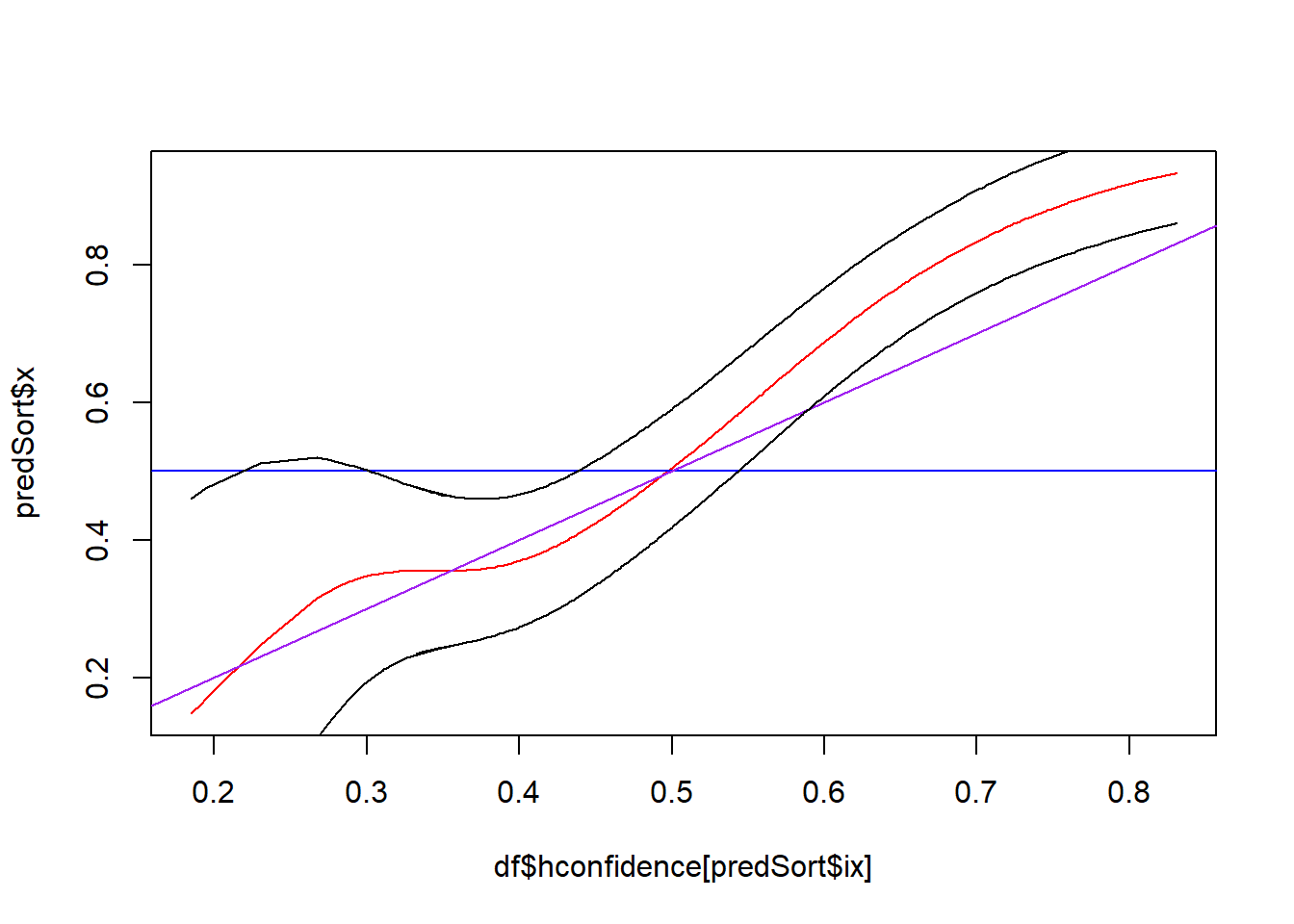
plot(predSort$x~df$hconfidence[predSort$ix],col="red",type="l")

abline(h=0.5,col="blue")
abline(v=50,col="blue")
abline(c(0,1),col="purple")
lines(df$hconfidence[predSort$ix],predSort$x+2*preds$se.fit[predSort$ix])
lines(df$hconfidence[predSort$ix],predSort$x-2*preds$se.fit[predSort$ix])
# predicting winners
ft=gam(I(actualhomemargin>0)~s(hconfidence),data=df,family="binomial",sp=0.05)
# the 0.05 was to make it a bit wiggly but not too silly (the default was not monotonically increasing, which is silly)
plot(ft,rug=FALSE,trans=binomial()$linkinv)
abline(h=0.5,col="blue")
abline(v=0.5,col="blue")
abline(c(0,1),col="purple")
# predicting margins
ft=gam(actualhomemargin~s(hconfidence),data=df)
plot(ft,rug=FALSE,residual=TRUE,pch=1,cex=0.4)
abline(h=0.5,col="blue")
abline(v=0.5,col="blue")

# add squiggle margins to the plot
confSort = sort(df$hconfidence,index.return=TRUE)
lines(confSort$x,df$squigglehomemargin[confSort$ix],col="purple")
[Read more...]

Punctuation in literature

June 29, 2018 | Rstats on Julia Silge

This morning I was scrolling through Twitter and noticed Alberto Cairo share this lovely data visualization piece by Adam J. Calhoun about the varying prevalence of punctuation in literature. I thought, “I want to do that!” It also offers me the opportunity to chat about a few of the new ... [Read more...]

Three Deep Truths About R

June 29, 2018 | William Doane

Everything that exists in R is an object ~ John M. Chambers Everything that happens in R is the result of a function call ~ John M. Chambers Names have objects; objects don’t have names ~ Hadley Wickham So, what are the implications of these statements? Everything in R is an object ... [Read more...]

Global Migration, animated with R

June 29, 2018 | David Smith

The animation below, by Shanghai University professor Guy Abel, shows migration within and between regions of the world from 1960 to 2015. The data and the methodology behind the chart is described in this paper. The curved bars around the outside represent the peak migrant flows for each region; globally, migration peaked ... [Read more...]

World Cup Analysis

June 29, 2018 | Stefan Musch

The grandest sports tournament on Earth is here, and that can only mean one thing: predictive modeling! Our model predicted 13 of 16 of the final teams correctly. Read on to find our prediction on who will win the 2018 World Cup!
[Read more...]

Farewell to Shiny Appreciation month

June 29, 2018 | Mango Solutions

As we come to the end of Shiny Appreciation month we hope that the blog posts and tweets have encouraged more of you to start using Shiny to create your own interactive web applications. If you need some help however with getting started with Shiny, or with more advanced functionality ... [Read more...]

Analyzing voter survey data with R

June 29, 2018 | Lesley Lathrop

I love polls. All kinds of polls, but especially political polls. I think I love them because I like politics and I also like to find out what’s going on in people’s heads, which is something that survey data allows one to do.So I was thrilled to ... [Read more...]

Comparing predictions: World Cup scores

June 29, 2018 | Jakob Gepp

As many others too, me and some colleges at STATWORX took part in a little betting game for the World Cup 2018. Since the group stage is over, I was wondering how well – or better – how worse my prediction was. I am comparing my result with other predictions by using the ...
[Read more...]

Beeswarms instead of histograms

June 28, 2018 | aghaynes

Histograms are good, density plots are also good. Violin and bean plots too. Recently I had someone ask for a plot where you could see each individual point along a continuum, give the points specific colours based on a second variable (similar to the figure), which deviates somewhat from the ...
[Read more...]
1 2 3 15

Never miss an update!
Subscribe to R-bloggers to receive
e-mails with the latest R posts.
(You will not see this message again.)

Click here to close (This popup will not appear again)