
Easy quick PCA analysis in R
Want to share your content on R-bloggers? click here if you have a blog, or here if you don't.
Principal component analysis (PCA) is very useful for doing some basic quality control (e.g. looking for batch effects) and assessment of how the data is distributed (e.g. finding outliers). A straightforward way is to make your own wrapper function for prcomp and ggplot2, another way is to use the one that comes with M3C (https://bioconductor.org/packages/devel/bioc/html/M3C.html) or another package. M3C is a consensus clustering tool that makes some major modifications to the Monti et al. (2003) algorithm so that it behaves better, it also provides functions for data visualisation.
Let’s have a go on an example cancer microarray dataset.
# M3C loads an example dataset mydata with metadata desx
library(M3C)
# do PCA
pca(mydata,colvec=c('gold'),printres=TRUE)
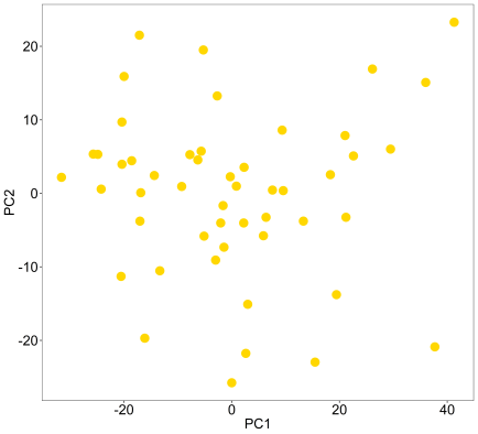
So, now what prcomp has done is extracted the eigenvectors of the data’s covariance matrix, then projected the original data samples onto them using linear combination. This yields PC scores which are plotted on PC1 and PC2 here (eigenvectors 1 and 2). The eigenvectors are sorted and these first two contain the highest variation in the data, but it might be a good idea to look at additional PCs, which is beyond this simple blog post and function.
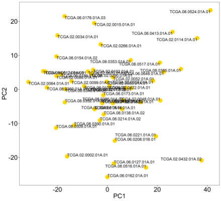
You can see above there are no obvious outliers for removal here, which is good for cluster analysis. However, were there outliers, we can label all samples with their names using the ‘text’ parameter.
library(M3C)
pca(mydata,colvec=c('gold'),printres=TRUE,text=colnames(mydata))
Now other objectives would be comparing samples with batch to make sure we do not have batch effects driving the variation in our data, and comparing with other variables such as gender and age. Since the metadata only contains tumour class we are going to use that next to see how it is related to these PC scores.
This is a categorical variable, so the ‘scale’ parameter should be set to 3, ‘controlscale’ is set to TRUE because I want to choose the colours, and ‘labels’ parameter passes the metadata tumour class into the function. I am increasing the ‘printwidth’ from its default value because the legend is quite wide.
For more information see the function documentation using ?pca.
# first reformat meta to replace NA with Unknown
desx$class <- as.character(desx$class)
desx$class[is.na(desx$class)] <- as.factor('Unknown')
# next do the plot
pca(mydata,colvec=c('gold','skyblue','tomato','midnightblue','grey'),
labels=desx$class,controlscale=TRUE,scale=3,printres=TRUE,printwidth=25)

So, now it appears that the variation that governs these two PCs is indeed related to tumour class which is good. But, what if the variable is continuous, and we wanted to compare read mapping rate, or read duplication percentage, or age with our data? So, a simple change of the parameters can allow this too. Let’s make up a continuous variable, then add this to the plot. In this case we change the ‘scale’ parameter to reflect we are using continuous data, and the spectral palette is used for the colours by default.
randomvec <- seq(1,50)
pca(mydata,labels=randomvec,controlscale=TRUE,scale=1,legendtitle='Random',
printres=TRUE,printwidth=25)
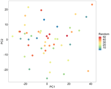
So, since this is a random variable, we can see it has no relationship with our data. Let’s just define a custom scale now. So we change ‘scale’ to 2, then use the ‘low’ and ‘high’ parameters to define the scale colour range.
pca(mydata,labels=randomvec,controlscale=TRUE,scale=2,legendtitle='Random',
printres=TRUE,,printwidth=25,low='grey',high='red')

Super easy, yet pretty cool. The idea here is just to minimise the amount of code hanging around for doing basic analyses like these. You can rip the code from here: https://github.com/crj32/M3C/blob/master/R/pca.R. Remember if your features are on different scales, the data needs transforming to be comparable beforehand.
M3C is part of a series of cluster analysis tools that we are releasing, the next is ‘Spectrum’, a fast adaptive spectral clustering tool, which is already on CRAN (https://cran.r-project.org/web/packages/Spectrum/index.html). Perhaps there will be time to blog about that in the future.
For quantitative analysis of drivers in the variation on data, I recommend checking out David Watson’s great function in the ‘bioplotr’ package called ‘plot_drivers’ (https://github.com/dswatson/bioplotr). This compares the PCs with categorical and continuous variables and performs univariate statistical analysis on them producing a very nice plot.
R-bloggers.com offers daily e-mail updates about R news and tutorials about learning R and many other topics. Click here if you're looking to post or find an R/data-science job.
Want to share your content on R-bloggers? click here if you have a blog, or here if you don't.