
Markov Switching Multifractal (MSM) model using R package
[This article was first published on K & L Fintech Modeling, and kindly contributed to R-bloggers]. (You can report issue about the content on this page here)
Want to share your content on R-bloggers? click here if you have a blog, or here if you don't.
This post explains the Markov switching multifractal (MSM) model of Calvet and Fisher (2004) and introduces a R package for this model. It is well-known that MSM model can describe stylized facts of volatility such as long memory, volatility clustering, and so on. Since It is a variant of Hamilton regime switching model with high-dimensional states, we can apply the same filtering approach except the probability transition matrix. Want to share your content on R-bloggers? click here if you have a blog, or here if you don't.
Markov Switching Multifractal model
Calvet and Fisher (2004) propose a discrete-time stochastic volatility model in which regime switching serves three purposes. First, changes in regimes capture low-frequency variations. Second, they specify intermediate-frequency dynamics usually assigned to smooth autoregressive transitions. Finally, high-frequency switches generate substantial outliers.
This multi-frequency regime switching model is called the Markov Switching Multifractal (MSM) model. MSM model tends to outperform major volatility models such as GARCH, MS-GARCH, FIGARCH and so on.
For readers who are not familiar with the regime switching model, there are some previous posts.
Univariate MSM model
The univariate Markov Switching Multifractal model is a stochastic volatility model in which conditional volatility is defined as a product of finitely many latent volatility state variables (called volatility components or frequency components), with varying degrees of persistence. Let \(r_t ≡ ln(\frac{P_t}{P_{ t− 1}})\). Then \(r_t\) is modeled as
\[\begin{align} r_t = \sigma(M_{1t}⨉M_{2t}⨉\ldots⨉M_{Kt})^{1/2} \epsilon_t \end{align}\]
where \(\epsilon_t\) is the i.i.d. standard normal distribution \(N(0,1)\) and \(\sigma\) is the unconditional volatility of returns. \(M_{kt}\) is determined by the following binomial distribution \(M\).
\[\begin{align} &M_{kt} \text{ drawn from } M &\text{ with prob } &\gamma_k \\ &M_{kt} = M_{k,t-1} &\text{ with prob } &1-\gamma_k \end{align}\]
The volatility components \(M_{kt}\) differ in their transition probabilities \(\gamma_k\) but not in their marginal distribution \(M\). The transition probabilities \(\gamma ≡ \left(\gamma_1, \gamma_2, …, \gamma_{K}\right)\) are specified as
\[\begin{align} \gamma_k = 1 – (1-\gamma_1)^{b^{k-1}} \end{align}\]
The univariate MSM(K) model is characterized by four parameters (\(m_0\),\(b\),\( \gamma_K\),\(\sigma\)),
- \(m_0 ∈ (1, 2]\) : the size of each volatility component
- \(b ∈ (1, ∞)\) : controls the probability of switching
- \(\gamma_{K} ∈ (0, 1)\): controls the spacing between different volatility components
- \(\sigma ∈ [0, ∞]\): the unconditional standard deviation
Given \(\gamma_{K}\),\(b\) as parameters and \(K\) as a hyper-parameter, we can recover \(\gamma_1, \gamma_2, …, \gamma_{K-1}\) as follows.
\[\begin{align} \gamma_{K} = 1 – (1-\gamma_1)^{b^{K-1}} \rightarrow \gamma_1 = 1 – (1 – \gamma_{K})^\frac{1}{b^{K-1}} \end{align}\]
Since the volatility state vector is \(M_t = (M_{1t}, M_{2t},\ldots,M_{Kt})\). MSM(K) model has \(2^K\) states and \(2^K \times 2^K\) transition probability matrix between each \(2^K\) states. It’s because K volatility components have two possible values (\(m_0\) and \(m_1 = 2-m_0\)). For example, when K=3, we can construct \(8(=2^3)\) states and \(8 \times 8\) transition probability matrix between each \(8\) states.
\(2^3\) states
\(2^3 \times 2^3\) transition probability matrix
|
Estimation of MSM model
Since MSM model is a kind of the regime-switching model, its parameters can be estimated via MLE with Hamilton filtering. This is the same procedure as that in the previous posts except some notations. When \(d=2^K\), this filtering repeats the following calculations n times (where n is the total number of observations in the dataset)
| 1) \(t-1\) state (previous state) \[\begin{align} \Pi_{t-1}^i = P(M_{t-1} = m^i|\tilde{r}_{t-1};\mathbf{\theta}) \end{align}\] 2) state transition from \(i\) to \(j\) (state propagation) \[\begin{align} P_{ij} = P(M_{t+1} = m^j | M_t = m^i),\quad 1 \le i,j \le d \end{align}\] 3) normal probability densities under j-regime at \(t\) \[\begin{align} f_{jt} &= N(r_t,\text{mean}=0, \text{sd}=\sigma_j) \end{align}\] 4) \(t\) posterior state (corrected from previous state) \[\begin{align} \Pi_{t} &= \frac{ f_t * (\Pi_{t-1}P) }{ [f_t * (\Pi_{t-1}P)]\iota^{\top} } \end{align}\] |
Here * denotes the element by element multiplication and \(\iota =(1,1,….,1)\). As a result of this filtering, the log likelihood can be calculated in the following way.
\[\begin{align} \log L(\tilde{r}_{t};\mathbf{\theta}) = \sum_{t=1}^{T}{ \log[f_t * (\Pi_{t-1}P)] } \end{align}\]
Install the MSM package from GitHub
Waleem Alausa kindly provides an R package for the Markov Switching Multifractal model (https://github.com/Waleem/MSM). This is located at GitHub repository so that we can install it in the following way.
- library(devtools)
- install_github(“Waleem/MSM”)
If devtools is not installed in advance, use the following command to install it from CRAN.
- install.packages(“devtools”)
R code
MSM R package contains the exchange rate dataset (level and return) which are used in Calvet and Fisher (2004). This exercise estimate conditional volatilities of Canadian dollar (CAD/USD) exchange rate. This series begin on June 1, 1974 and run until June 30, 2002, which contains 7049 observations.
The following R code estimates parameters of a MSM(3) model and decomposes this conditional volatility series into its volatility components using MSM R package and also shows an example of forecasting.
#========================================================# # Quantitative ALM, Financial Econometrics & Derivatives # ML/DL using R, Python, Tensorflow by Sang-Heon Lee # # https://kiandlee.blogspot.com #——————————————————–# # MSM model #========================================================# #library(devtools) #install_github(“Waleem/MSM”) library(MSM) graphics.off() # clear all graphs rm(list = ls()) # remove all files from your workspace #————————————— # Data used in Calvet and Fisher (2004) #————————————— data(“calvet2004data”) ret <– na.omit(as.matrix(calvet2004data$caret)) #————————————— # MSM estimation #————————————— kbar <– 3 fit <– Msm(ret, kbar=kbar, n.vol=252, nw.lag=2) df.est <– cbind(fit$coefficients, fit$se) df.est #————————————— # fitted volatility #————————————— fitted <– predict.msmmodel(fit) vol_fit <– fitted$vol*sqrt(252) #————————————— # decomposition of volatility components #————————————— em <– Msm_decompose(fit) #————————————— # graph : return, abs(ret), fitted volatility #————————————— x11(); par(mfrow=c(4,1), mar=c(2,2,2,2)) plot(ret, main = “return (daily)”, type = “l”) plot(abs(ret), main = “absolute return (daily)”, type = “l”) plot(vol_fit, main = “MSM volatility”, col = “blue”, type = “l”, lwd = 2) matplot(cbind(abs(ret)*sqrt(252), vol_fit), type = “l”, main = “absolute return*sqrt(252) vs MSM volatility”, col = c(“grey”,“blue”), lty = 1, lwd = c(1,2)) #————————————— # volatility component #————————————— x11(); par(mfrow=c(kbar,1), mar=c(2,2,2,2)) for (i in 1:kbar) { plot(em[,i], type = “l”, main = paste0(“volatility component “, i)) } #————————————— # forecast #————————————— vol_forecast <– predict.msmmodel(fit, h = 7) | cs |
The following figures show the estimated parameters and a conditional time series of volatility estimates with return data.

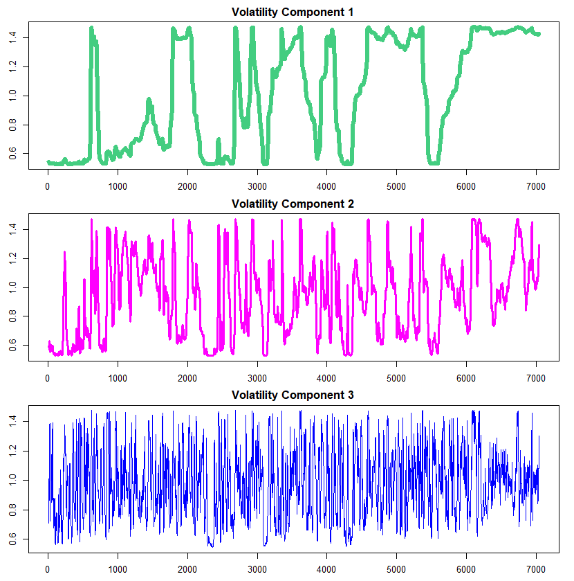
The above conditional volatility can be decomposed into three (=K) volatility components which are depicted in the figures below. As can be seen easily, the 3rd component is least persistent and 1st component most persistent. In particular the 2nd component exhibits a kind of autoregressive behavior. These differences result from the different frequencies by which heterogeneous regime changes may occur.
Concluding Remarks
This post explained the univariate MSM volatility model and implemented it by using Waleem Alausa’s MSM R package. There is also the bivariate MSM model which incorporate multi-frequency correlations between two assets. This bivariate MSM model is somewhat difficult to implement it but this R package also provide this model. \(\blacksquare\)
Reference
Calvet, L. E. and A. J. Fisher (2004) How to Forecast Long-run Volatility: Regime Switching and the Estimation of Multifractal Processes. Journal of Financial Econometrics 2-1, 49-83.
To leave a comment for the author, please follow the link and comment on their blog: K & L Fintech Modeling.
R-bloggers.com offers daily e-mail updates about R news and tutorials about learning R and many other topics. Click here if you're looking to post or find an R/data-science job.
Want to share your content on R-bloggers? click here if you have a blog, or here if you don't.