It is Sunday, it's raining and I have a few hours to spend before I am invited for lunch at my parents place. Hence, I thought I'd use the time to produce another post. It has been a while since the last post as I have been in Africa for about two months for yet another stint of fieldwork on the great Kilimanjaro mountain…

This time I want to introduce the strip() function which is part of the METVURST suite for plotting meteorological/climatological data (available from https://github.com/tim-salabim/metvurst)

This function is intended to facilitate two things:

1. to enable plotting of large (climatological) data sets at hourly resolution (the data need to be hourly observations) in a reasonably well defined space (meaning that you won't need pages and pages of paper to print the results).
2. to display the data in a way that interpretation is possible from hourly to decadal time scales.

The function is much like the calendarHeat() function from Revolution Analytics (see here) though, as mentioned above, it produces plots of hourly data. In fact, calendarHeat() would be a good alternative to use when you intend to plot daily values.
strip() is implemented in lattice (needs latticeExtra to be more precise) and essentially plots a levelplot of hour of day (y-axis) vs. day of year (x-axis).

In detail the function takes the following parameters:

• x (numeric): Object to be plotted (e.g. temperature).
• date (character or POSIXct): Date(time) of the observations. Format must be 'YYYY-MM-DD hh:mm(:ss)'
• fun: The function to be used for aggregation to hourly observations (if original is of higher frequency). Default is mean.
• cond (factor): Conditioning variable e.g. years.
• arrange (character): One of “wide” or “long”. Defaults to “long” which provides a layout that is easier to interpret, however, “wide” is better for use in presentation slides.
• colour (character): a vector of color names. Defaults to rev(brewer.pal(11, “Spectral”))
• …: Further arguments to be passed to levelplot (see ?lattice::levelplot for options). This can be quite handy to set the legend title using main = "YOUR TEXT HERE" (the legend is plotted on top of the actual plot).

Here's an example using hourly data from Fiji (Station is at Lautoka on the west coast). The data can be freely accessed through the Bureau of Meteorology in Australia (BOM).

First we need to download the data and do some reshaping

## LOAD RColorBrewer FOR COLOR CREATION
library(RColorBrewer)

## SET URL FOR DATA DOWNLOAD
url <- "http://www.bom.gov.au/ntc/IDO70004/IDO70004_"

## YEARS TO BE DOWNLOADED
yr <- 1993:2012

## READ DATA FOR ALL YEARS FROM URL INTO LIST
fijilst <- lapply(seq(yr), function(i) {
  read.csv(paste(url, yr[i], ".csv", sep = ""), na.strings = c(-9999, 999))
  })

## TURN LIST INTO COMPLETE DATAFRAME AND CONVERT NA STRINGS TO NAs
fiji <- do.call("rbind", fijilst)
fiji[fiji == -9999.00] <- NA
fiji[fiji == -9999.0] <- NA
fiji[fiji == 999.0] <- NA

## CREATE POSIX DATETIME AND CONVERT UTC TO LOCAL FIJI TIME
dts <- as.POSIXct(strptime(fiji$Date...UTC.Time, 
                  format = "%d-%b-%Y %H:%M")) + 12 * 60 * 60

## CREATE CONDITIONING VARIABLE (IN THIS CASE YEAR)
year <- substr(as.character(dts), 1, 4)

Now, let's plot the temperatures

## SOURCE FUNCTION (ALSO AVAILABLE AT https://github.com/tim-salabim/metvurst)
source("http://www.staff.uni-marburg.de/~appelhat/r_stuff/strip.R")

## PLOT STRIP FOR TEMPERATURE
strip(x = fiji$Air.Temperature, 
      date = dts,
      cond = year,
      arrange = "long",
      main = "Temperature")

## 
##  Module   :  strip 
##  Author   :  Tim Appelhans <[email protected]>, Thomas Nauss 
##  Version  :  2012-01-06 
##  License  :  GNU GPLv3, see http://www.gnu.org/licenses/

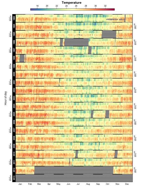
We can clearly see both the diurnal and the seasonal signal.
Looking at other parameters such as wind direction and speed should also give an interesting insight into the seasonal and diurnal dynamics of the location.

I leave it up to you to explore this further…

I am off to a nice sunday roast now! yumyum

sessionInfo()

## R version 2.15.3 (2013-03-01)
## Platform: x86_64-pc-linux-gnu (64-bit)
## 
## locale:
##  [1] LC_CTYPE=en_US.UTF-8       LC_NUMERIC=C              
##  [3] LC_TIME=en_US.UTF-8        LC_COLLATE=en_US.UTF-8    
##  [5] LC_MONETARY=en_US.UTF-8    LC_MESSAGES=en_US.UTF-8   
##  [7] LC_PAPER=C                 LC_NAME=C                 
##  [9] LC_ADDRESS=C               LC_TELEPHONE=C            
## [11] LC_MEASUREMENT=en_US.UTF-8 LC_IDENTIFICATION=C       
## 
## attached base packages:
## [1] grid      parallel  stats     graphics  grDevices utils     datasets 
## [8] methods   base     
## 
## other attached packages:
##  [1] reshape_0.8.4       plyr_1.8            latticeExtra_0.6-19
##  [4] lattice_0.20-13     RColorBrewer_1.0-5  RWordPress_0.2-3   
##  [7] rgdal_0.8-5         raster_2.0-41       sp_1.0-5           
## [10] knitr_1.1          
## 
## loaded via a namespace (and not attached):
## [1] digest_0.6.3   evaluate_0.4.3 formatR_0.7    markdown_0.5.4
## [5] RCurl_1.95-3   stringr_0.6.2  tools_2.15.3   XML_3.95-0    
## [9] XMLRPC_0.2-5