
visualising diurnal wind climatologies
Want to share your content on R-bloggers? click here if you have a blog, or here if you don't.
In this post I want to highlight the second core function of the metvurst repository (https://github.com/tim-salabim/metvurst):
The windContours function
It is intended to provide a compact overview of the wind field climatology at a location and plots wind direction and speed as a function of the hour of day.
- direction is plotted as frequencies of occurrences
- speed is represented by a box plot
The classical approach for visualising wind direction and speed at a location is to plot a wind rose where a stacked barplot of speeds is plotted in a circular coordinates system showing the direction. As an example of a wind rose we take the example from the Wikipedia page for “wind rose”.

This kind of representation is very useful for getting a general sense of the of the wind field climatology at a location.
You will be able to quickly get information along the lines of. “the x most prevailing wind directions are from here, there and sometimes also over there”. Furthermore, you will also know which of these tends to produce windier conditions. So far, so good.
If you want to learn about possible diurnal flow climatologies, however, there is no way of obtaining this information straight from the wind rose. The common way to achieve visualising such dynamics using wind roses is to plot individual roses for some specific period (e.g. hourly or 3 hourly roses).
Getting information on diurnal climate dynamics is especially important in regions of complex terrain or for coastal locations, where diurnally reversing wind flow patterns are a major climatic feature.
The windContours function is able to deliver such information at a glance.
Consider the case from the last post, where we used hourly meteorological information from a coastal station in Fiji.
First, we (again) read the data from the web at BOM (Australian Bureau Of Meteorology).
## LOAD RColorBrewer FOR COLOR CREATION
library(metvurst)
library(RColorBrewer)

## SET URL FOR DATA DOWNLOAD
url <- "http://www.bom.gov.au/ntc/IDO70004/IDO70004_"

## YEARS TO BE DOWNLOADED
yr <- 1993:2012

## READ DATA FOR ALL YEARS FROM URL INTO LIST
fijilst <- lapply(seq(yr), function(i) {
 read.csv(paste(url, yr[i], ".csv", sep = ""), na.strings = c(-9999, 999))
})

## TURN LIST INTO COMPLETE DATAFRAME AND CONVERT NA STRINGS TO NAs
fiji <- do.call("rbind", fijilst)
fiji[fiji == -9999] <- NA
fiji[fiji == -9999] <- NA
fiji[fiji == 999] <- NA

## CREATE POSIX DATETIME AND CONVERT UTC TO LOCAL FIJI TIME
dts <- as.POSIXct(strptime(fiji$Date...UTC.Time,
 format = "%d-%b-%Y %H:%M")) + 12 * 60 * 60
Next, we need to create a vector of the hours of the recordings in order to plot our hourly climatologies.
## CREATE CONDITIONING VARIABLE (IN THIS CASE HOUR)
hr <- substr(as.character(dts), 12, 13)
Now, we can use the windContours function straight away to plot the hourly wind direction frequencies and corresponding wind speeds for the observation period 1993 – 2012.
Note, for reproducibility I have posted the function on my personal uni web page, but it is recommended that you get the function from the metvurst repository at git hub.
windContours(hour = hr,
             wd = fiji$Wind.Direction,
             ws = fiji$Wind.Speed,
             keytitle = "hourly wind frequencies [%]")
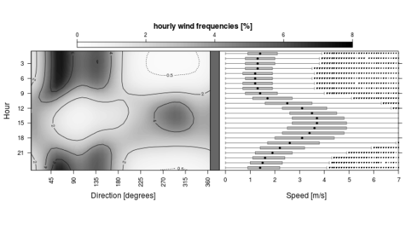
Just as we would with a wind rose, we easily see that there are 3 main prevailing wind directions:
- north north-east
- south-east
- west north-west
However, we straight away realise that there is a distinct diurnal pattern in these directions with 1. and 2. being nocturnal and 3. denoting the daytime winds. This additional information is captured at a glance.
It is possible to refine the graph in a lot of ways.
In the next few figures I want to highlight a few of the flexibilities that windContours provides:
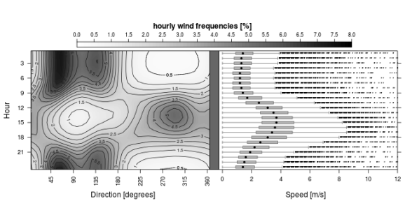
In order to adjust the x-axis of the speed plot, use the speedlim = parameter
windContours(hour = hr,
             wd = fiji$Wind.Direction,
             ws = fiji$Wind.Speed,
             speedlim = 12,
             keytitle = "hourly wind frequencies [%]")

In case you want to change the density of the contour lines you can use spacing =
windContours(hour = hr,
             wd = fiji$Wind.Direction,
             ws = fiji$Wind.Speed,
             speedlim = 12,
             keytitle = "hourly wind frequencies [%]",
             spacing = .5)
You can also provide colors through the colour = parameter
windContours(hour = hr,
             wd = fiji$Wind.Direction,
             ws = fiji$Wind.Speed,
             speedlim = 12,
             keytitle = "hourly wind frequencies [%]",
             colour = rev(brewer.pal(11, "Spectral")))

You can adjust the number of cuts to be made using ncuts =
windContours(hour = hr,
             wd = fiji$Wind.Direction,
             ws = fiji$Wind.Speed,
             speedlim = 12,
             keytitle = "hourly wind frequencies [%]",
             colour = rev(brewer.pal(11, "Spectral")),
             ncuts = .5)
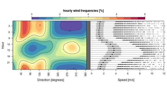
Apart from the design, you can also adjust the position of the x-axis so that the plot is centered north (default is south) using the centre = parameter (allowed values are: “S”, “N”, “E”, “W”)
windContours(hour = hr,
             wd = fiji$Wind.Direction,
             ws = fiji$Wind.Speed,
             speedlim = 12,
             keytitle = "hourly wind frequencies [%]",
             colour = rev(brewer.pal(11, "Spectral")),
             centre = "N")

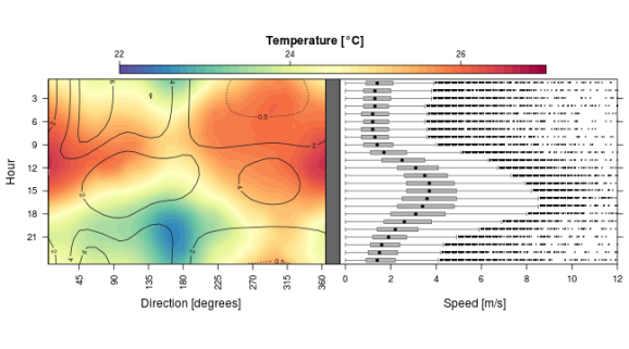
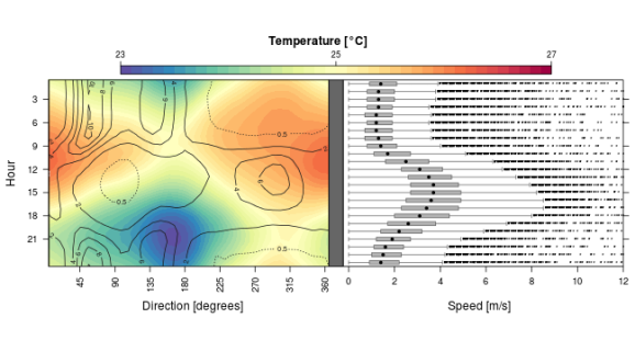
There’s also the possibility to provide an additional variable using add.var = in order to examine the relationship between winds and some other parameter of interest (e.g. concentrations of some pollutant or precipitation or anything really). In doing so, the contours will remain as before (representing wind direction frequencies) and the (colour-)filled part of the left panel will be used to represent the additional variable.
Here, we’re using air temperature (don’t forget to change the keytitle) where we can easily see that cold air mainly comes from south (extra-tropical air masses) and highest temperatures are observed when air flow is from northerly directions (tropical air masses)
windContours(hour = hr,
             wd = fiji$Wind.Direction,
             ws = fiji$Wind.Speed,
             speedlim = 12,
             keytitle = "Temperature [°C]",
             colour = rev(brewer.pal(11, "Spectral")),
             add.var = fiji$Air.Temperature)
In case you want to change the smoothing of the contours you can use the smooth.contours = parameter.
The same applies to the (colour-)filled area using smooth.fill =
windContours(hour = hr,
             wd = fiji$Wind.Direction,
             ws = fiji$Wind.Speed,
             speedlim = 12,
             keytitle = "Temperature [°C]",
             colour = rev(brewer.pal(11, "Spectral")),
             add.var = fiji$Air.Temperature,
             smooth.contours = .8,
             smooth.fill = 1.5)
In the future I might present some analytical post making use of the windContours function to highlight its usefulness in climate analysis.
For now, I refer the interested reader to Appelhans et al. (2012) where I’m presenting the seasonal wind climatology of Christchurch, New Zealand and also analyse general diurnal patterns of air pollution using windContours.
sessionInfo()
## R version 2.15.3 (2013-03-01)
## Platform: x86_64-pc-linux-gnu (64-bit)
##
## locale:
##  [1] LC_CTYPE=en_US.UTF-8       LC_NUMERIC=C
##  [3] LC_TIME=en_US.UTF-8        LC_COLLATE=en_US.UTF-8
##  [5] LC_MONETARY=en_US.UTF-8    LC_MESSAGES=en_US.UTF-8
##  [7] LC_PAPER=C                 LC_NAME=C
##  [9] LC_ADDRESS=C               LC_TELEPHONE=C
## [11] LC_MEASUREMENT=en_US.UTF-8 LC_IDENTIFICATION=C
##
## attached base packages:
## [1] grid      parallel  stats     graphics  grDevices utils     datasets
## [8] methods   base
##
## other attached packages:
##  [1] gridBase_0.4-6      abind_1.4-0         fields_6.7
##  [4] spam_0.29-2         reshape_0.8.4       plyr_1.8
##  [7] latticeExtra_0.6-19 lattice_0.20-13     RColorBrewer_1.0-5
## [10] RWordPress_0.2-3    rgdal_0.8-5         raster_2.0-41
## [13] sp_1.0-5            knitr_1.1
##
## loaded via a namespace (and not attached):
## [1] digest_0.6.3   evaluate_0.4.3 formatR_0.7    markdown_0.5.4
## [5] RCurl_1.95-3   stringr_0.6.2  tools_2.15.3   XML_3.95-0
## [9] XMLRPC_0.2-5

R-bloggers.com offers daily e-mail updates about R news and tutorials about learning R and many other topics. Click here if you're looking to post or find an R/data-science job.
Want to share your content on R-bloggers? click here if you have a blog, or here if you don't.