
Working with Venn Diagrams
Want to share your content on R-bloggers? click here if you have a blog, or here if you don't.
In this post, we will learn how to create venn diagrams for gene lists and how to retrieve the genes present in each venn compartment with R.
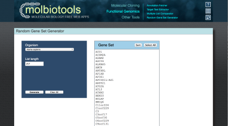
In this particular example, we will generate random gene lists using the molbiotools gene set generator but you can use your own gene lists if you prefer. Specifically, we will generate a random list of 257 genes to represent those that are upregulated in condition and another list of 1570 genes to represent those that are upregulated in condition B.
Then, we will sort and paste the gene lists in an excel document we will save as randomGeneLists.xlsx.
Now, let’s load the data into R using the gdata package.
library("gdata")
geneLists <- read.xls("randomGeneLists.xlsx", sheet=1, stringsAsFactors=FALSE, header=FALSE)
head(geneLists)

# Notice there are empty strings to complete the data frame in column 1 (V1)
tail(geneLists)

# To convert this data frame to separate gene lists with the empty strings removed we can use lapply() with our home made  function(x) x[x != ""]
geneLS <- lapply(as.list(geneLists), function(x) x[x != ""])

# If this is a bit confusing you can also write a function and then use it in lapply()
removeEMPTYstrings <- function(x) {

 newVectorWOstrings <- x[x != ""]
 return(newVectorWOstrings)

}
geneLS2 <- lapply(as.list(geneLists), removeEMPTYstrings)

# You can print the last 6 entries of each vector stored in your list, as follows:
lapply(geneLS, tail)
lapply(geneLS2, tail) # Both methods return the same results

# We can rename our list vectors
names(geneLS) <- c("ConditionA", "ConditionB")

# Now we can plot a Venn diagram with the VennDiagram R package, as follows:
require("VennDiagram")

VENN.LIST <- geneLS
venn.plot <- venn.diagram(VENN.LIST , NULL, fill=c("darkmagenta", "darkblue"), alpha=c(0.5,0.5), cex = 2, cat.fontface=4, category.names=c("A", "B"), main="Random Gene Lists")

# To plot the venn diagram we will use the grid.draw() function to plot the venn diagram
grid.draw(venn.plot)

# To get the list of gene present in each Venn compartment we can use the gplots package
require("gplots")

a <- venn(VENN.LIST, show.plot=FALSE)

# You can inspect the contents of this object with the str() function
str(a)

# By inspecting the structure of the a object created,
# you notice two attributes: 1) dimnames 2) intersections
# We can store the intersections in a new object named inters
inters <- attr(a,"intersections")

# We can summarize the contents of each venn compartment, as follows:
# in 1) ConditionA only, 2) ConditionB only, 3) ConditionA & ConditionB
lapply(inters, head)

Now you are ready, to review the genes in each section of the venn diagram separately. Alternatively, you can always use Venny web tool that is a great way to start looking at your data and then write a modified version of this R script to make a more exhaustive figure or facilitate downstream analysis in your script.
Feel free to leave comments or email me at [email protected].

R-bloggers.com offers daily e-mail updates about R news and tutorials about learning R and many other topics. Click here if you're looking to post or find an R/data-science job.
Want to share your content on R-bloggers? click here if you have a blog, or here if you don't.