Veterinary Epidemiologic Research: Modelling Survival Data – Non-Parametric Analyses
Want to share your content on R-bloggers? click here if you have a blog, or here if you don't.
Next topic from Veterinary Epidemiologic Research: chapter 19, modelling survival data. We start with non-parametric analyses where we make no assumptions about either the distribution of survival times or the functional form of the relationship between a predictor and survival. There are 3 non-parametric methods to describe time-to-event data: actuarial life tables, Kaplan-Meier method, and Nelson-Aalen method.
We use data on occurrence of calf pneumonia in calves raised in 2 different housing systems. Calves surviving to 150 days without pneumonia are considered censored at that time.
temp <- tempfile()
download.file(
"http://ic.upei.ca/ver/sites/ic.upei.ca.ver/files/ver2_data_R.zip", temp)
load(unz(temp, "ver2_data_R/calf_pneu.rdata"))
unlink(temp)

library(Hmisc)
calf_pneu <- upData(calf_pneu, labels = c(calf = 'Calf id',
                                  stock = 'Stocking method',
                             days = 'Time to onset of pneumonia or censoring',
                                  pn = 'Pneumonia'),
                  levels = list(stock = list('batch' = 0, 'continuous' = 1)))
Actuarial Life Table
To create a life table, we use the function lifetab from package KMsurv, after calculating the number of censored and events at each time point and grouping them by time interval (with gsummary from package nlme).
library(KMsurv)
interval <- seq(from = 30, to = 165, by = 15)
interval <- floor(calf_pneu$days/15)
interval.censor <- data.frame(interval, calf_pneu$pn)
library(nlme)
pneumonia <- gsummary(interval.censor, sum, groups = interval)
total <- gsummary(interval.censor, length, groups = interval)
lt.data <- cbind(pneumonia[ , 1:2], total[ , 2])
length <- length(lt.data$interval)
lt.data[length + 1, ]$interval <- NA
nevent <- lt.data[ , 2]
nlost <- lt.data[ , 3] - lt.data[ , 2]
(life.table <- lifetab(lt.data$interval, 24, nlost, nevent))
      nsubs nlost nrisk nevent      surv        pdf     hazard    se.surv
1-3      24     0  24.0      1 1.0000000 0.02083333 0.02127660 0.00000000
3-4      23     0  23.0      1 0.9583333 0.04166667 0.04444444 0.04078938
4-5      22     0  22.0      1 0.9166667 0.04166667 0.04651163 0.05641693
5-6      21     0  21.0      3 0.8750000 0.12500000 0.15384615 0.06750772
6-7      18     1  17.5      2 0.7500000 0.08571429 0.12121212 0.08838835
7-8      15     6  12.0      3 0.6642857 0.16607143 0.28571429 0.09686316
8-10      6     0   6.0      1 0.4982143 0.04151786 0.09090909 0.11032937
10-NA     5     5   2.5      0 0.4151786         NA         NA 0.11915934
NA-3      0    NA    NA     NA 0.4151786         NA         NA 0.11915934
          se.pdf  se.hazard
1-3   0.02039469 0.02127178
3-4   0.04078938 0.04443347
4-5   0.04078938 0.04649905
5-6   0.06750772 0.08855994
6-7   0.05792828 0.08555236
7-8   0.08649471 0.16326531
8-10  0.03899969 0.09053265
10-NA         NA         NA
NA-3          NA         NA
Kaplan-Meier Method
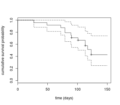
To compute the Kaplan-Meier estimator we use the function survfit from package survival. It takes as argument a Surv object, which gives the time variable and the event of interest. You get the Kaplan-Meier estimate with the summary of the survfit object. We can then plot the estimates to show the Kaplan-Meier survivor function.
library(survival)
km.sf <- survfit(Surv(days, pn == 1) ~ 1, data = calf_pneu)
summary(km.sf)
Call: survfit(formula = Surv(days, pn == 1) ~ 1, data = calf_pneu)

 time n.risk n.event survival std.err lower 95% CI upper 95% CI
   27     24       1    0.958  0.0408        0.882        1.000
   49     23       1    0.917  0.0564        0.813        1.000
   72     22       1    0.875  0.0675        0.752        1.000
   79     21       2    0.792  0.0829        0.645        0.972
   89     19       1    0.750  0.0884        0.595        0.945
   90     18       1    0.708  0.0928        0.548        0.916
  101     17       1    0.667  0.0962        0.502        0.885
  113     15       2    0.578  0.1019        0.409        0.816
  117      9       1    0.514  0.1089        0.339        0.778
  123      6       1    0.428  0.1198        0.247        0.741

plot(km.sf, xlab = "time (days)", ylab = "cumulative survival probability", conf.int = TRUE)
Nelson-Aalen Method
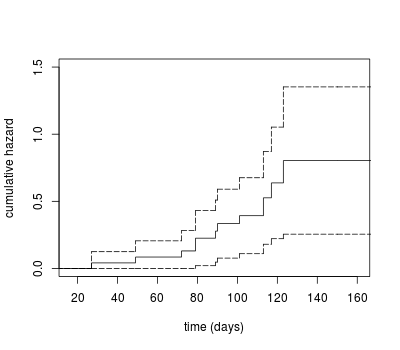
A “hazard” is the probability of failure at a point in time, given that the calf had survived up to that point in time. A cumulative hazard, the Nelson-Aaalen estimate, can be computed. The Nelson-Aalen estimate can be calculated by transforming the Fleming-Harrington estimate of survival.
fh.sf <- survfit(Surv(days, pn == 1) ~ 1, data = calf_pneu, type = "fleming")

plot(stepfun(fh.sf$time, c(0, -log(fh.sf$surv))), do.points = FALSE,
      xlab = "time (days)", ylab = "cumulative hazard",
      main = "", ylim = c(0, 1.5))
lines(stepfun(fh.sf$time, c(0, -log(fh.sf$upper))), lty = 5, do.points = FALSE)
lines(stepfun(fh.sf$time, c(0, -log(fh.sf$lower))), lty = 5, do.points = FALSE)
Tests of the Overall Survival Curve
Several tests are available to test whether the overall survivor functions in 2 or more groups are equal. We can use the log-rank test, the simplest test, assigning equal weight to each time point estimate and equivalent to a standard Mantel-Haenszel test. Also, there’s the Peto-Peto-Prentice test which weights the stratum-specific estimates by the overall survival experience and so reduces the influence of different censoring patterns between groups.
To do these tests, we apply the survdiff function to the Surv object. The argument rho gives the weights according to and may be any numeric value. Default is rho = 0 which gives the log-rank test. Rho = 1 gives the “Peto & Peto modification of the Gehan-Wilcoxon test”. Rho larger than zero gives greater weight to the first part of the survival curves. Rho smaller than zero gives weight to the later part of the survival curves.
survdiff(Surv(days, pn == 1) ~ stock, data = calf_pneu, rho = 0) # rho is optional
Call:
survdiff(formula = Surv(days, pn == 1) ~ stock, data = calf_pneu,
    rho = 0)

                  N Observed Expected (O-E)^2/E (O-E)^2/V
stock=batch      12        4     6.89      1.21      2.99
stock=continuous 12        8     5.11      1.63      2.99

 Chisq= 3  on 1 degrees of freedom, p= 0.084

survdiff(Surv(days, pn == 1) ~ stock, data = calf_pneu, rho = 1) # rho=1 asks for Peto-Peto test
Call:
survdiff(formula = Surv(days, pn == 1) ~ stock, data = calf_pneu,
    rho = 1)

                  N Observed Expected (O-E)^2/E (O-E)^2/V
stock=batch      12     2.89     5.25      1.06      3.13
stock=continuous 12     6.41     4.05      1.38      3.13

 Chisq= 3.1  on 1 degrees of freedom, p= 0.0766
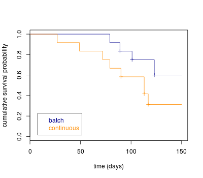
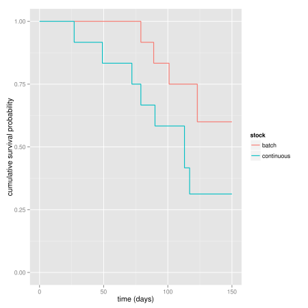
Finally we can compare survivor function with stock R plot or using ggplot2. With ggplot2, you get the necessary data from the survfit object and create a new data frame from it. The baseline data (time = 0) are not there so you create it yourself:
(km.stock <- survfit(Surv(days, pn == 1) ~ stock, data = calf_pneu))
Call: survfit(formula = Surv(days, pn == 1) ~ stock, data = calf_pneu)

                 records n.max n.start events median 0.95LCL 0.95UCL
stock=batch           12    12      12      4     NA     123      NA
stock=continuous      12    12      12      8    113      79      NA

plot(km.stock, conf.int = FALSE, col = c("blue4", "darkorange"),
      xlab = "time (days)", ylab = "cumulative survival probability")
legend("bottomleft", inset = .05, c("batch", "continuous"),
        text.col = c("blue4", "darkorange"))

km.df <- data.frame(
    time    = km.stock$time,
    n.risk  = km.stock$n.risk,
    n.event = km.stock$n.event,
    surv    = km.stock$surv,
    strata  = gsub("stock=", "", summary(km.stock, censored = T)$strata),
    upper   = km.stock$upper,
    lower   = km.stock$lower
 )
zeros <- data.frame(time = 0, surv = 1, strata = gsub("stock=", "",
                                           levels(summary(km.stock)$strata)),
                     upper = 1, lower = 1)
library(plyr)
km.df <- rbind.fill(zeros, km.df)
km.df$strata <- ordered(km.df$strata, levels = c("batch", "continuous"))
library(ggplot2)
ggplot(km.df, aes(time, surv, colour = strata)) +
   geom_step(size = 0.6) + xlim(0, 150) + ylim(0, 1) +
   xlab("time (days)") + ylab("cumulative survival probability") +
   labs(colour = "stock")
R-bloggers.com offers daily e-mail updates about R news and tutorials about learning R and many other topics. Click here if you're looking to post or find an R/data-science job.
Want to share your content on R-bloggers? click here if you have a blog, or here if you don't.


