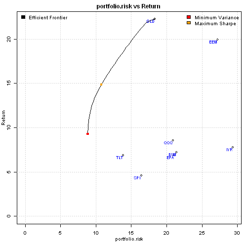
Maximum Sharpe Portfolio or Tangency Portfolio is a portfolio on the efficient frontier at the point where line drawn from the point (0, risk-free rate) is tangent to the efficient frontier.

There is a great discussion about Maximum Sharpe Portfolio or Tangency Portfolio at quadprog optimization question. In general case, finding the Maximum Sharpe Portfolio requires a non-linear solver because we want to find portfolio weights w to maximize w' mu / sqrt( w' V w ) (i.e. Sharpe Ratio is a non-linear function of w). But as discussed in the quadprog optimization question, there are special cases when we can use quadratic solver to find Maximum Sharpe Portfolio. As long as all constraints are homogeneous of degree 0 (i.e. if we multiply w by a number, the constraint is unchanged – for example, w1 > 0 is equivalent to 5*w1 > 5*0), the quadratic solver can be used to find Maximum Sharpe Portfolio or Tangency Portfolio.

I have implemented the logic to find Maximum Sharpe Portfolio or Tangency Portfolio in the max.sharpe.portfolio() function in strategy.r at github. You can specify following 2 parameters:

• Type of portfolio: ‘long-only’, ‘long-short’, or ‘market-neutral’
• Portfolio exposure. For example, ‘long-only’ with exposure = 1, is a fully invested portfolio

Now, let’s construct a sample efficient frontier and plot Maximum Sharpe Portfolio.

###############################################################################
# Load Systematic Investor Toolbox (SIT)
# http://systematicinvestor.wordpress.com/systematic-investor-toolbox/
###############################################################################
setInternet2(TRUE)
con = gzcon(url('http://www.systematicportfolio.com/sit.gz', 'rb'))
    source(con)
close(con)
 
	#*****************************************************************
	# Create Efficient Frontier
	#****************************************************************** 	
	# create sample historical input assumptions
	ia = aa.test.create.ia()
	
	# create long-only, fully invested efficient frontier
	n = ia$n		

	# 0 <= x.i <= 1
	constraints = new.constraints(n, lb = 0, ub = 1)
		constraints = add.constraints(diag(n), type='>=', b=0, constraints)
		constraints = add.constraints(diag(n), type='<=', b=1, constraints)
		
	# SUM x.i = 1
	constraints = add.constraints(rep(1, n), 1, type = '=', constraints)		
	
	# create efficient frontier
	ef = portopt(ia, constraints, 50, 'Efficient Frontier') 
	
	#*****************************************************************
	# Create Plot
	#****************************************************************** 	
	# plot efficient frontier
	plot.ef(ia, list(ef), transition.map=F)	 
	
	# find maximum sharpe portfolio
	max(portfolio.return(ef$weight,ia) /  portfolio.risk(ef$weight,ia))
	
	# plot minimum variance portfolio
	weight = min.var.portfolio(ia,constraints)	
	points(100 * portfolio.risk(weight,ia), 100 * portfolio.return(weight,ia), pch=15, col='red')
	portfolio.return(weight,ia) /  portfolio.risk(weight,ia)
		
	# plot maximum Sharpe or tangency portfolio
	weight = max.sharpe.portfolio()(ia,constraints)	
	points(100 * portfolio.risk(weight,ia), 100 * portfolio.return(weight,ia), pch=15, col='orange')
	portfolio.return(weight,ia) /  portfolio.risk(weight,ia)
		
	plota.legend('Minimum Variance,Maximum Sharpe','red,orange', x='topright')	

Now let’s see how to construct ‘long-only’, ‘long-short’, or ‘market-neutral’ Maximum Sharpe Portfolio or Tangency Portfolios:

	#*****************************************************************
	# Examples of Maximum Sharpe or Tangency portfolios construction
	#****************************************************************** 	
	weight = max.sharpe.portfolio('long-only')(ia,constraints)	
		round(weight,2)
		round(c(sum(weight[weight<0]), sum(weight[weight>0])),2)
		
	weight = max.sharpe.portfolio('long-short')(ia,constraints)			
		round(weight,2)
		round(c(sum(weight[weight<0]), sum(weight[weight>0])),2)
		
	weight = max.sharpe.portfolio('market-neutral')(ia,constraints)			
		round(weight,2)
		round(c(sum(weight[weight<0]), sum(weight[weight>0])),2)	

The long-only Maximum Sharpe portfolio as expected has exposure of 100%. The long-short Maximum Sharpe portfolio is 227% long and 127% short. The market-neutral Maximum Sharpe portfolio is 100% long and 100% short.

As the last step, I run Maximum Sharpe algo vs other portfolio optimization methods I have previously discussed (i.e. Risk Parity, Minimum Variance, Maximum Diversification, Minimum Correlation) on the 10 asset universe used in the Adaptive Asset Allocation post.

	#*****************************************************************
	# Load historical data
	#****************************************************************** 
	load.packages('quantmod')
	
	tickers = spl('SPY,EFA,EWJ,EEM,IYR,RWX,IEF,TLT,DBC,GLD')

	data <- new.env()
	getSymbols(tickers, src = 'yahoo', from = '1980-01-01', env = data, auto.assign = T)
		for(i in ls(data)) data[[i]] = adjustOHLC(data[[i]], use.Adjusted=T)							
	bt.prep(data, align='keep.all', dates='2004:12::')
 
	#*****************************************************************
	# Code Strategies
	#******************************************************************
	prices = data$prices  
	n = ncol(prices)
   
	models = list()
   
 	#*****************************************************************
	# Code Strategies
	#******************************************************************
	# find period ends
	period.ends = endpoints(prices, 'months')
        period.ends = period.ends[period.ends > 0]
        
	n.mom = 180
	n.vol = 60
	n.top = 4        
	momentum = prices / mlag(prices, n.mom)  
       
	obj = portfolio.allocation.helper(data$prices, period.ends=period.ends,
		lookback.len = n.vol, universe = ntop(momentum[period.ends,], n.top) > 0,
		min.risk.fns = list(EW=equal.weight.portfolio,
						RP=risk.parity.portfolio,
						MV=min.var.portfolio,
						MD=max.div.portfolio,
						MC=min.corr.portfolio,
						MC2=min.corr2.portfolio,
						MCE=min.corr.excel.portfolio,
						MS=max.sharpe.portfolio())
	) 
	
	models = create.strategies(obj, data)$models
					
	#*****************************************************************
	# Create Report
	#******************************************************************    
	strategy.performance.snapshoot(models, T)

	plotbt.custom.report.part2(models$MS)

	# Plot Portfolio Turnover for each strategy
	layout(1)
	barplot.with.labels(sapply(models, compute.turnover, data), 'Average Annual Portfolio Turnover')

The allocation using Maximum Sharpe Portfolio produced more concentrated portfolios with higher total return, higher Sharpe ratio, and higher turnover.