
How to perform consensus clustering without overfitting and reject the null hypothesis
Want to share your content on R-bloggers? click here if you have a blog, or here if you don't.
The Monti et al. (2003) consensus clustering algorithm is one of the most widely used class discovery techniques in the genome sciences and is commonly used to cluster transcriptomic, epigenetic, proteomic, and a range of other types of data. It can automatically decide the number of classes (K), by resampling the data and for each K (e.g. 2-10) calculating a consensus rate of how frequently each pair of samples are sampled together by a given clustering algorithm, e.g. PAM. These consensus rates form a consensus matrix. A perfect consensus matrix for any given K would just consist of 0s and 1s because all samples always cluster together or not together over all resampling iterations. Whereas values around 0.5 would indicate the clustering is less clear. However, as Șenbabaoğlu et al. (2014) recently pointed out, consensus clustering is subject to false discoveries, like many clustering algorithms are, as they usually do not test the null hypothesis K=1 (no structure). We also found the consensus clustering algorithm overfits, this is why we developed M3C which was inspired by the GAP-statistic.
M3C (https://bioconductor.org/packages/release/bioc/html/M3C.html) uses a multicore Monte Carlo simulation, that maintains the correlation structures of the features of the input data, to make multivariate Gaussian references for consensus clustering to eliminate overfitting. We use the reference relative Relative Cluster Stability Index (RCSI) and p values to chose K and reject the null hypothesis K=1. The package also contains a variety of other functions and features for investigating data, such as PCA, tSNE, automatic clinical data analysis, and a selection of clustering algorithms we have tested such as PAM, k-means, self-tuning spectral clustering, and Ward’s hierarchal clustering.
Let’s take a look at a demonstration and show how it removes the limitations of the method. This is with the developers’ version of M3C which comes with a glioblastoma cancer dataset with tumor classes (from histology) labeled in a description object.
library(M3C)
dim(mydata) # we have 1740 features and 50 samples (microarray data)
[1] 1740   50
head(desx) # we have a annotation file with tumour types labelled
class                  ID
TCGA.02.0266.01A.01         TCGA.02.0266.01A.01
TCGA.08.0353.01A.01   Proneural TCGA.08.0353.01A.01
TCGA.06.0175.01A.01 Mesenchymal TCGA.06.0175.01A.01
TCGA.08.0346.01A.01 Mesenchymal TCGA.08.0346.01A.01
TCGA.02.0114.01A.01   Proneural TCGA.02.0114.01A.01
TCGA.02.0048.01A.01   Proneural TCGA.02.0048.01A.01
So now we know something about the data we are working with we can go ahead and run M3C. This code just uses the default algorithm, PAM, and in this case we are setting the ‘doanalysis’ and ‘analysistype’ parameters to get M3C to analyze the clinical data we are inputting. Since the variable we want to test for is categorical, we can do a chi-squared test. The ‘printres’ parameter will get all our results printed in the current directory.
res <- M3C(mydata,des=desx,cores=2,doanalysis=TRUE,analysistype='chi',
printres = TRUE)
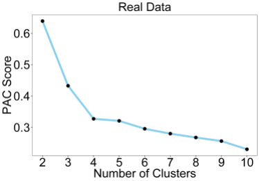
This plot shows the PAC score, which is a measure of consensus matrix stability for each value of K. A PAC score of 0 indicates perfect clustering. As we can see, there is a trend towards lower values of K, which is an overfitting effect. This is commonly observed on real datasets with the PAC score, although it performs better than the original delta K. Delta K is still commonly used to this day despite performing poorly simply because there are so many publications which have used it in the past. The PAC score overfitting effect can be eliminated by using the RCSI which takes the reference into account.
We can see the RCSI below, removes the overfitting effect and a maximum (which indicates the optimal K) is found for K=4.

M3C also calculates empirical p values from the reference distributions to test the null hypothesis K=1. We can see below, for both K=4 and K=5 we can reject the null hypothesis K=1.

These are the results quantified in a table. The beta p value is simply where the N Monte Carlo simulations were used to yield the parameters required for a theoretical beta distribution from which a p value can be derived that may go lower than those provided by 100 Monte Carlo iterations. We chose a beta distribution because the reference distributions for K=2 often exhibit skew and kurtosis. The PAC score also occurs in the range 0-1, the same as the beta distribution. The chi-squared test in the below table tells us K=4 and K=5 are two optimal values for the relationship of the clinical data with the discovered classes. There are some NA values due to incomplete data.
We can see from the significant relationship of the clinical data, particularly with the M3C optimal K, that the framework works.
res$scores
K  PAC_REAL   PAC_REF         RCSI MONTECARLO_P     BETA_P   P_SCORE
1  2 0.6391837 0.5722939 -0.110539221   0.69306931 0.65102440 0.1864027
2  3 0.4326531 0.5602776  0.258496125   0.09900990 0.09587818 1.0182802
3  4 0.3273469 0.4847918  0.392699013   0.02970297 0.01060788 1.9743716
4  5 0.3208163 0.4149796  0.257360575   0.04950495 0.02856676 1.5441390
5  6 0.2955102 0.3602776  0.198171342   0.05940594 0.05211127 1.2830683
6  7 0.2800000 0.3150857  0.118055107   0.15841584 0.16558430 0.7809809
7  8 0.2677551 0.2796735  0.043549978   0.30693069 0.35994732 0.4437610
8  9 0.2563265 0.2523020 -0.015825197   0.55445545 0.56868102 0.2451313
9 10 0.2302041 0.2282449 -0.008547061   0.49504950 0.54129058 0.2665695

> res$clinicalres
K          chi
1  2 8.977979e-07
2  3 2.482780e-11
3  4 1.806709e-13
4  5 7.124742e-13
5  6 1.294080e-11
6  7          NaN
7  8          NaN
8  9          NaN
9 10          NaN
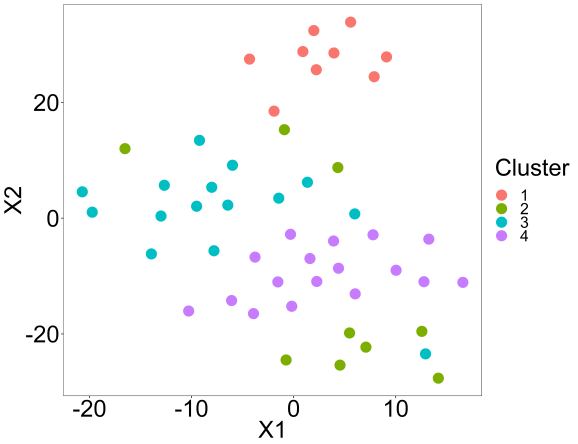
Lastly, we can perform a tsne analysis with the package to visually confirm the clusters.
tsne(res,K=4,perplex=10,printres=TRUE)
Summary
We have seen in this blog post how the M3C package provides a powerful approach to identifying classes using consensus clustering in high dimensional continuous data. I suggest trying the approach and comparing it with others for yourself. We have also included a simple data simulator in the package to encourage user testing of class discovery methods used in the field of cancer research and stratified medicine. A more complex data simulator has been made in parallel with M3C called, ‘clusterlab’ on CRAN (https://cran.r-project.org/web/packages/clusterlab/index.html). This method offers precise control over variance, spacing, outliers, and cluster size. Together, these tools provide a framework for the detection of classes for precision medicine and in other fields.
R-bloggers.com offers daily e-mail updates about R news and tutorials about learning R and many other topics. Click here if you're looking to post or find an R/data-science job.
Want to share your content on R-bloggers? click here if you have a blog, or here if you don't.