
Example 8.25: more latent class models (plus a graphical display)
[This article was first published on SAS and R, and kindly contributed to R-bloggers]. (You can report issue about the content on this page here)
Want to share your content on R-bloggers? click here if you have a blog, or here if you don't.
Want to share your content on R-bloggers? click here if you have a blog, or here if you don't.
In recent entries (here, here, here and here), we’ve been fitting a series of latent class models using SAS and R. One of the most commonly used and powerful package for latent class model estimation is Mplus. In this entry, we demonstrate how to use the MplusAutomation package to automate the process of fitting and interpreting a series of models using Mplus.
The first chunk of code needs to be run on a Windows computer with Mplus installed. We undertake the same analytic steps as before, then run the prepareMplusData() function to create the dataset, then createModels() to create the Mplus input files.
ds = read.csv("http://www.math.smith.edu/r/data/help.csv")
attach(ds)
library(MplusAutomation)
cesdcut = ifelse(cesd>20, 1, 0)
smallds = na.omit(data.frame(homeless, cesdcut,
  satreat, linkstatus))
prepareMplusData(smallds, file="mplus.dat")
createModels("mplus.txt")
Once the preliminaries have been completed, we can run each of the models, then scarf up the results.
runModels()
summary=extractModelSummaries()
models=readModels()
To help create graphical summaries of the classes, I crafted some code that utilizes the Mplus output files. These include functions to calculate the antilogit (alogit()), determine class probabilities in terms of model parameters (calcclasses() and findprobs()), and a routine to plot the resulting values (plotres()). Unfortunately, these routines require tweaking for models with different number of predictors (as well as care if some of the predictors have more than 2 levels).
alogit = function(x) {
        return(exp(x)/(1+exp(x)))
}

calcclasses = function(vals) {
   numvals = length(vals)
   classes = numeric(numvals+1)
   for (i in 1:numvals) {
      classes[i] = exp(vals[i])/
         (1+sum(exp(vals[1:numvals])))
   }
   classes[numvals+1] = 1/(1+sum(exp(vals[1:numvals])))
   return(classes)
}

findprobs = function(df) {
   numclass = length(levels(as.factor(df$LatentClass)))-1
   v1 = numeric(numclass)
   v2 = numeric(numclass)
   v3 = numeric(numclass)
   v4 = numeric(numclass)
   for (i in 1:numclass) {
      v1[i] = alogit(-df$est[4*(i-1)+1])
      v2[i] = alogit(-df$est[4*(i-1)+2])
      v3[i] =  alogit(-df$est[4*(i-1)+3])
      v4[i] =  alogit(-df$est[4*(i-1)+4])
   }
   if (numclass>1) {
      classes=calcclasses(df$est[(4*numclass+1):(4*numclass+numclass-1)])
   } else classes=1
   return(list(prop=cbind(v1=v1, v2=v2, v3=v3, v4=v4),
     classes=classes))
}

plotres = function(mylist, roundval=1, cexval=.75) {
# can only plot at most 4 classes!
   reorder = order(mylist$classes)
   probs = mylist$classes[reorder]
   results = mylist$prop
   dimen = dim(results)
   cols = c(1,4,2,5) # black, blue, red, and turquoise
   ltys = c(3,1,2,4) # dotted, solid, dash, dash-dot
   ltyslines = ltys[rank(-mylist$classes)]
   colslines = cols[rank(-mylist$classes)]
   ltysrev = rev(ltys[1:dimen[1]])
   colsrev = rev(cols[1:dimen[1]])
   plot(c(0.9, dimen[2]), c(-0.08,1), xlab="",
           ylab="estimated prevalence", xaxt="n", type="n")
   abline(h=0, col="gray")
   abline(h=1, col="gray")
   for (i in 1:(dimen[1])) {
      lines(1:(dimen[2]), results[i,], lty=ltyslines[i],
         col=colslines[i], lwd=2)
      points(1:(dimen[2]), results[i,], col=colslines[i])
   }
   text(1,0,"homeless", pos=1, cex=cexval)
   text(2,0,"cesdcut", pos=1, cex=cexval)
   text(3,0,"satreat", pos=1, cex=cexval)
   text(4,0,"linkstat", pos=1, cex=cexval)
   legendval = character(dimen[1])
   for (i in 1:(dimen[1])) {
      legendval[i] = paste("class ",i , " (", round(100*probs[i],
         roundval), "%)", sep="")
   }
   legend(2, 0.4, legend=legendval,
      lty=ltysrev, col=colsrev, cex=cexval, lwd=2)
}
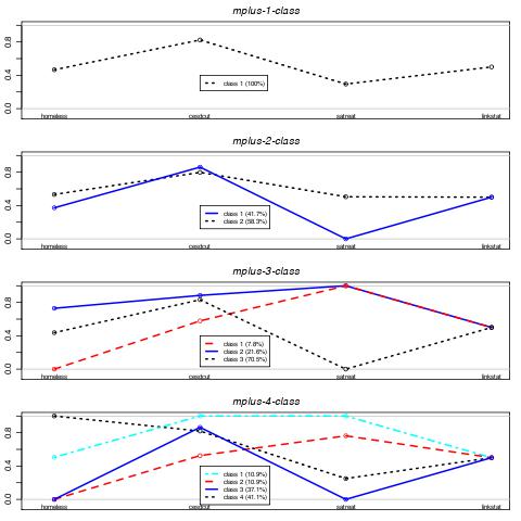
Finally, by spelunking through the output files in the current directory (using list.files()) the results from each of the four models can be collated and displayed as seen in the Figure above.
The single class model simply reproduces the prevalences of each of the predictors. The two class solution primarily separates those not receiving substance abuse treatment from those that do. The three class solution further splits along substance abuse treatment, as well as homeless status. The four class solution is somewhat jumbled, with a group of homeless subjects comprising the largest class. None of the classes distinguish linkstatus (the primary outcome of the RCT).
To leave a comment for the author, please follow the link and comment on their blog: SAS and R.
R-bloggers.com offers daily e-mail updates about R news and tutorials about learning R and many other topics. Click here if you're looking to post or find an R/data-science job.
Want to share your content on R-bloggers? click here if you have a blog, or here if you don't.