Hello, I hope you have your Yorkshire tea ready as today I am going to be exploring weighted averages using R.

bb3_sum = bb1 %>% mutate(wick = if_else(filt == "bowled", "bowled", 
                                if_else(filt == "caught", "caught", 
                                if_else(filt == "caught and bowled", "caught and bowled", 
                                if_else(filt == "handled the ball", "handled the ball", 
                                if_else(filt == "hit wicket", "hit wicket", 
                                if_else(filt == "lbw", "lbw", 
                                if_else(filt == "run out", "run out", 
                                if_else(filt == "stumped", "stumped", NA_character_))))))))) %>%
                                mutate(wickno = if_else(is.na(wick), 0, 1)) %>%
                                left_join(bb2_CLEAN, by = "file") %>%
                                filter(season == 2022) %>%
                                bat_run2 = as.numeric(as.character(bat_run))) %>%
                                group_by(bat) %>%
                                summarise(totrun = sum(bat_run2), totwick = sum(wickno)) %>%
                                mutate(Batting_Average = round(totrun/totwick,2)) %>%
                                            select(bat, totrun, Batting_Average) %>%
                                                    filter(totrun > 200) %>%
                                                      slice_max(Batting_Average, n = 15) %>%
                             rename("Batter" = bat, "Total Runs" = totrun, "Batting Average" = Batting_Average)



library(gt)



bat_av_tab = gt(bb3_sum) %>%
                   tab_header(
    title = md("**County Championship 2022 Batting Averages**"),
    subtitle = md("The *top 15* players are shown")
  )
 

I used the code above to generate the table of the top 15 players by batting average in the 2022 county championship. Now the whole point of this blog is to devise a weighted average and see the comparison

Weighted Average? what?

One of the key metrics in cricket, for a batter especially, is their batting average. Now weighted averages have been spoken about in this article on Cricinfo [1] however this just describes adjusting the batting average to account for the impact of not outs. I envisage a weighted average controlling for the quality of the bowling attack and the quality of the pitch. This looks to be what the England cricket team use [2] and a methodology has been defined for international cricket in this blog here [3]

In the example above of 2 players, one averaging in the 30s and the other averaging in the lower 20s. If you were a selector for a team, player A would be selected based on that data alone.

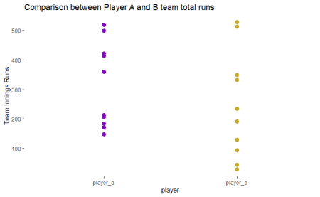
Well, above you can see the total scores for the whole innings for each of the players. It looks like player a has actually batted in innings that scored higher. In reality, both these players are of the same quality they are both average batters. Hence using a weighted average will make these comparisons fairer.

Method

The methodology is split into 2 parts controlling for the quality of the pitch and the quality of the bowling attack.

#### calcuting the average player score depending on the total for the teams

play_tots_all =  bb1 %>% mutate(bat_run = as.numeric(as.character(bat_run))) %>%
                      group_by(file, team, mi, bat) %>%
                       summarise(tot_run = sum(bat_run)) %>%
                          left_join(bb3, by = c("file", "team", "mi")) %>%
                              group_by(tot_run_t) %>%
                                summarise(averu = mean(tot_run))

# calculating the average player score for the average team total 

play_tots_all_av = play_tots_all %>%
                                ungroup() %>%
                                    summarise(meanav = mean(averu), meanin = mean(tot_run_t))


# adding the average player score and runs and calcuting the % difference

play_tots_all2 = play_tots_all %>% 
                              bind_cols(play_tots_all_av) %>%
                                        mutate(avedelt = 1-averu/meanav) %>%
                                  filter(avedelt > -2)

## plotting the result 

ggplot(play_tots_all2, aes(x = tot_run_t, y = avedelt)) + geom_point(col = "#12006b", alpha = 0.7) +
                                                            geom_smooth(method = "lm", col = "#f07229", se = F) +
      labs(x = "Team Total Runs", 
           y = "% Difference to Average Score",
         title = "Difference to Player Average by Team Total Runs") +
                                                              theme(panel.background = element_blank())  

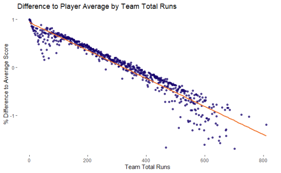
Above is how the difference to the average score that the average batter will score is impacted by the total runs a player will score.

### calculating the bowling average of all the bowlers in the data set 


bowlers = bb1 %>% mutate(wick = if_else(filt == "bowled", "bowled", 
                                    if_else(filt == "caught", "caught", 
                                      if_else(filt == "caught and bowled", "caught and bowled", 
                                        if_else(filt == "handled the ball", "handled the ball", 
                                          if_else(filt == "hit wicket", "hit wicket", 
                                            if_else(filt == "lbw", "lbw", 
                                              if_else(filt == "run out", NA_character_, 
                                                if_else(filt == "stumped", "stumped", NA_character_))))))))) %>%
                                      mutate(wickno = if_else(is.na(wick), 0, 1)) %>%
                                                mutate(tot_run = as.numeric(as.character(totrun))) %>%
                                                group_by(bowl) %>%
                                        summarise(total_run = sum(tot_run), tot_wick = sum(wickno), n = n()) %>%
                                                    mutate(bowlav = total_run/tot_wick) %>%
                                                        filter(tot_wick > 0) %>%
                                                          filter(n > 100)



# working out the average bowling average of all the bowlers who boled in the innigs


bowl_qual = bb1 %>% left_join(bowlers, by = "bowl") %>%
                        mutate(tot_run = as.numeric(as.character(totrun))) %>%
                          group_by(team, mi, file) %>%
                              summarise(inntot = sum(tot_run), bowlq = mean(bowlav, na.rm = T))



# calculating the average score and bowl quality

bowl_qual2 = bowl_qual %>% ungroup() %>%
                              summarise(meansc = mean(inntot), meanq = mean(bowlq, na.rm=T))


# working out the difference to the average 

bowl_qual3 = bowl_qual %>% bind_cols(bowl_qual2) %>%
                                    mutate(indelt = inntot/meansc-1, bowlqr = round(bowlq, 1)) %>%
                                      group_by(bowlqr) %>%
                                        summarise(delta = mean(indelt)) %>%
                                          filter(bowlqr < 41)


## plotting the result

ggplot(bowl_qual3, aes(x = bowlqr, y = delta)) + geom_point(col = "#f07229", size = 2) +
                                                            geom_smooth(method = "lm", col = "#12006b", se = F) +
                      labs(x = "Bowling Quality", y = "% Impact on Score", title = "Impact of the QUality of the Bowling Attack on Score", subtitle = "Bowling quality of the average Bowling avrage of all the bowlers in the innings") +
                                                              theme(panel.background = element_blank())  

Above is the impact the quality of the bowling attack has on the score of the team. Now that I have my two regression lines for the impact the pitch and bowling attack have on a team I can apply these to every inning from every player in the dataset to make the adjusted runs scored and subsequently average.

# creating the two linnear regression models 
ave_play = lm(avedelt~tot_run_t, play_tots_all2)




lm2_bowl = lm(delta ~ bowlqr, bowl_qual3)

## creating the dataset with all batters there total runs scored per innings and the assiciated bowl quality and team total 

player_st = bb1 %>% 
                      mutate(bat_run2 = as.numeric(as.character(bat_run))) %>%
                                                          group_by(bat, team, mi, file) %>%
                                                              summarise(totrun = sum(bat_run2)) %>%
                                                     left_join(bb3, by = c("file", "mi", "team")) %>%
                                                          left_join(bowl_qual, by = c("file", "mi", "team")) %>%
                                                        rename("bowlqr" = bowlq, )



## generating the predictions
pred_team = predict(ave_play, player_st)


pred_bowl = predict(lm2_bowl, player_st)


## putting the predictions together with the innings data, 
player_st2 = player_st %>% bind_cols(pred_team) %>%
                            bind_cols(pred_bowl) %>%
                                  rename("run_delt" = ...11, "bowl_delt" = ...12) %>%
                                mutate(avdelt = (run_delt+bowl_delt)/2) %>%
                                  mutate(adj_runs = totrun * (1+avdelt))

The code above generates the table and now I can use the avdelt column which is the average of the impact of the pitch and the bowling attack to adjust the runs the player scored.

Results

The fun part the actual results from the new calculation. On the table, you can see the top 15 batters from the actual average but now with their newly calculated weighted average. The biggest loser for the players with multiple innings was Jennings who has had a 20 run reduction in his average – he must have scored his runs at easier times

Focusing in on a particular player we have Ben Duckett here who made the top 15 list from 2022. In all seasons before 2022, he often averaged around the low 40s and there was not too much difference in his weighted average. In the latest season 2022 he performed exceptionally well and this lead to his Englan recall.

As a metric, I think this does have more value than the traditional batting average. By being able to control for the quality of pitches and bowling attacks the number will have more value when used to compare players in a selection/recruitment scenario. one area I think my version could be refined would be to control for the different seasons. The last season in 2022 saw lots more runs scored than previous seasons.

References

[1] https://www.espncricinfo.com/story/the-weighted-batting-average-wba-in-tests-1225928

[2] https://uk.sport.cricket.narkive.com/M0C7Hwot/england-selection-by-numbers

[3] https://medium.com/@himanishganjoo/contextual-averages-a-new-way-of-looking-at-batting-in-cricket-a83803111b0e