This is the supplement to Chapter 5 of my book, Goals-Based Portfolio Theory, demonstrating the techniques and offering some code examples. If you are reading this having not purchased/read the book, you are missing much of the narrative. You can pick up a copy from Wiley, Amazon.com, or Barnes & Noble.

Now that we have established that goals-based investors have to think about risk differently than institutional investors, let’s dig into a couple of ways goals-based investors might think about managing risk.

When are Losses Too Much?

The first method for managing these unique goal-based investment risks is to use your goal variables to inform when portfolio losses are too much to recover from. This is a unique risk to goals-based investors because we have a time horizon, whereas institutional investors do not! The question is not whether markets recover, but whether they recover in time for you to achieve your goal.

A framework for thinking about this problem is ascertaining your portfolio’s maximum allowable loss (this is a simplified version which does not account for contributions—the full version, and its basic derivation, is in the book):

Where W is the amount of money needed to fund the goal, t is the number of years until you need the money, w is the amount of money you have dedicated to the goal today, and R is the recovery return you can expect from markets after a loss-making year.

Using R, we can visualize our portfolio’s maximum allowable loss, given various inputs.

# Load our libraries
library(tidyverse)

# Build Simplified Max Loss Function
maximum_loss.f <- function(w, W, t, R){
  W / (w * (R+1)^(t-1) ) - 1
}

# Show how time affects loss tolerance
t <- seq(5, 20, 0.5)

# Build viz
data.frame( 't' = t,
            'Max.Loss' = maximum_loss.f(0.65, 1, t, 0.12)) %>% 
  ggplot(., aes(x = t, y = Max.Loss)) +
  geom_line( size = 1.25 )+
  xlab('Time Until Goal')+
  ylab('')+
  ggtitle('Maximum Allowable Loss')

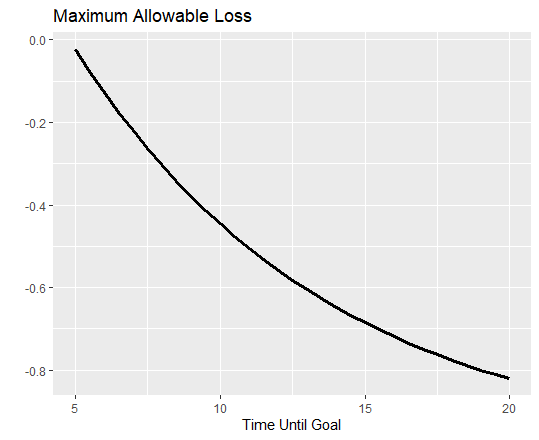
And so, we have a very simplistic framework for thinking about maximum losses for our goals-based portfolio.

Upside Risk vs Downside Risk

The method above, however, only addresses downside risk. Investors who make an active bet and move their portfolios to cash take a risk that markets move higher and leave them behind. This is upside risk. Balancing upside risk with downside risk is an important part of managing goals-based portfolios. But, how can we think about this balance?

If we think about a stop-loss strategy using the maximum allowable loss from above as our threshold, we can expect to exit our portfolio when our max loss is getting close to being violated. Then, we need to think about neutralizing our upside risk as quickly as possible.

A simple framework might be:

Where I is the percent of our portfolio that we need to reinvest, S is the price we stopped out at (the price we sold), B is our desired breakeven price, and P is our buy-back-in price.

Here’s what is going on: our breakeven price is the price at which we must buy back in lest we lose money because markets moved higher without us. By default, that price is the price at which we exit. However, when we buy back in, that price moves. We can set an arbitrary value here, but something like 10% to 20% higher than our exit price would give us some breathing room, as an example.

Assuming, then, that we have some market outlook (if we don’t, then this whole exercise is moot), we can balance our downside risk with the same variables:

where L is the expected portfolio loss, I is the percent we invest from here, and G is the expected portfolio loss still to go.

Using these two equations, we can begin thinking about balancing upside and downside risk. Let’s set up the problem in R:

# Function for % Invested for downside risk
invested_downside.f <- function(L, G){
  L / G
}

# Function for % Invested for upside risk
invested_upside.f <- function(S, B, P){
  (S - B)/(P - B)
}

# Set up a visulazation, using some assumptions
P <- seq(0.65, 1.00, 0.01) # Price is our variable
data.frame( 'Price' = c(P, # Set up x-axis
                        P),
            
            'Invested' = c( invested_downside.f( # Determine % To Invest to mitigate downside risk
                              maximum_loss.f(0.60, 1, 6, 0.12), # Using the maximum allowable loss from above
                              0.65-P), # And the amount of loss yet to go (mkt outlook)
                            # Determine % To Invest to neutralize upside risk:
                            invested_upside.f( 1.00, 1.20, P ) ), # Assuming we exited at 1.00 and we want 
                                                                  # our breakeven to be 20% higher
            
            'Type' = c( rep( 'Downside Risk', length(P)),
                        rep( 'Upside Risk', length(P) ) ) ) %>% 
  
  # Generate visualization
  ggplot(., aes(x = Price, y = Invested, lty = Type ))+
  geom_line( size = 1.25 )+
  ylim(0, 1)+
  ylab('% To Invest')

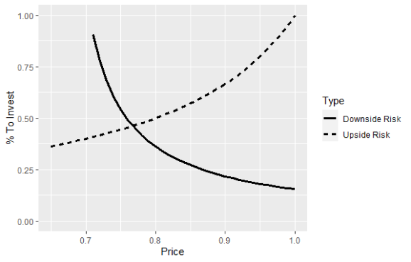
And here we can see the point at which upside risk and downside risk are equalized. Using these variables, we could invest 48% of the portfolio at around $0.77, and thereby neutralize our upside and downside risk at the same time. So long as we buy back in with the remainder of the portfolio at $1.20 or less, we are ahead on the trade. Of course, that does not mean we can sit back and declare victory, because our market outlook could well be wrong! In that case, we have to manage the portfolio through it (or accept this as a risk and move forward anyway).

Again, this is a very simplistic way to think about the problem, but it does at least open a line of thinking on the issue of managing downside and upside risk in a portfolio. And notice—none of this has anything at all to do with you psychological risk tolerance, this is entirely driven by what we expect from markets, and what we need markets to do for you!

Paying for Hedges

Another way to consider managing risks in a goals-based portfolio is to outright hedge it. Of course, when we talk about hedges, we now have to ask “what are you willing to pay for that protection?” And that is where things get a bit tricky.

Leaving the narrative for the book, let’s set up the problem in R:

phi.f <- function(x, location, scale){
  1 - 1 / ( 1 + exp( -(x-location)/scale ) )
}

loss_return <- -0.40
amount_of_max_loss <- -0.25
initial_wealth <- 0.75
required_wealth <- 1.00
time_until_goal <- 10
typical_return <- 0.08
typical_vol <- 0.11
recovery_return <- 0.10
recovery_vol <- 0.09
p <- 0.45


optim.f <- function(cost){
  
  # R_L is the recovery return needed in a non-hedged portfolio that experienced a loss.
  R_L <- (required_wealth/((1+loss_return)*initial_wealth) )^(1/(time_until_goal - 1)) - 1
  # R is the return needed after a typical year with no hedge
  R <- (required_wealth/( (1+typical_return)*initial_wealth ) )^(1/(time_until_goal - 1)) - 1
  # R_HL is the return needed after a loss-year with a hedge.
  R_HL <- (required_wealth / ( (1+amount_of_max_loss) * (initial_wealth + cost)))^(1/(time_until_goal - 1)) - 1
  # R_H is the return needed after paying for a hedge in a typical year.
  R_H <- (required_wealth / ( (1+typical_return) * (initial_wealth + cost)))^(1/(time_until_goal - 1)) - 1
  
  phi_L <- phi.f( R_L, recovery_return, recovery_vol )
  phi_R <- phi.f( R, typical_return, typical_vol )
  phi_HL <- phi.f( R_HL, recovery_return, recovery_vol )
  phi_H <- phi.f( R_H, typical_return, typical_vol )
  
  abs(p * phi_HL + (1-p) * phi_H - p * phi_L - (1-p) * phi_R)
  
}

prob <- seq(0.01, 0.65, 0.01)
c <- 0
for(i in 1:length(prob)){
  p <- prob[i]
  c[i] <- optim( -0.01, optim.f )$par
}

loss_return <- -0.30
amount_of_max_loss <- -0.15
c_2 <- 0
for(i in 1:length(prob)){
  p <- prob[i]
  c_2[i] <- optim( -0.01, optim.f )$par
}

time_until_goal <- 5
loss_return <- -0.40
amount_of_max_loss <- -0.15
c_3 <- 0
for(i in 1:length(prob)){
  p <- prob[i]
  c_3[i] <- optim(-0.01, optim.f )$par
}

data.frame( 'P' = c(prob,
                    prob,
                    prob),
            'C' = c(c,
                    c_2,
                    c_3),
            'Label' = c( rep('Scenario A', length(prob)),
                         rep('Scenario B', length(prob)),
                         rep('Scenario C', length(prob )))) %>% 
  ggplot( ., aes(x=P, y = C, color = Label))+
  geom_line( size = 1.25 )+
  scale_color_manual( values = c('black', 'grey', 'grey50'))+
  xlab('Probability of Bad Year')+
  ylab('Fair Value Cost to Hedge')+
  theme_minimal()+
  theme( axis.title = element_text(size = 16, face = 'bold'),
         axis.text = element_text( size = 14 ),
         legend.title = element_blank(),
         legend.text = element_text( size = 16, face = 'bold'),
         legend.position = 'top')

As we can clearly see, our willingness to pay for hedges depends quite a lot on our goal variables, as well as our market outlook! And none of it has to do with you psychological comfort with downside or upside. It has only to do with the intersection of what you need your portfolio to do and our market outlook.

These are some very simple frameworks for thinking about managing risk in a goals-based portfolio, however, there is much work yet to be done. In the end, goals-based investing is showing us that risk management is individuated, but that there are some ways to think about the problem rationally.