In a hospital, 9% of all patients have Covid-19. But: Among the heavy smokers among these patients, only 6% have Covid-19. What? Does smoking reduce your risk of getting Covid?

Another example: I recently saw a post on Twitter with a line graph showing that, in the UK, persons aged 18 to 59 who were vaccinated against the coronavirus had a higher risk of dying (from any cause) in the next 21 days as opposed to unvaccinated persons aged 18 to 59. Does the vaccine increase your chance of dying?

The answers to these questions can be found below. Let’s first try to understand what might be wrong with these two examples.

Why does correlation not imply causation?

By now you certainly have heard of the phrase “correlation does not imply causation”. So what does imply causation? In general, randomized control trials (RCT) are considered the gold standard for causal inference in science. If you were able to recruit a group of 10,000 non-smokers, randomly divide them into two groups, force the first group to start smoking heavily and the other to refrain from it, and observe the number of covid infections in both groups over the following months, you could be quite confident to identify a causal effect of smoking on the risk of catching covid with a simple comparison of counts and maybe a t-test for statistical significance. Here, correlation does imply causation.

[Just to be sure: Having a randomized experiment is no panacea to prevent every kind of statistical problem that might arise; for instance, is your sample size large enough; is your sample representative of the population of interest; are your measurements valid and reliable, etc. But in terms of possible distortions from third variables, RCT’s are the best way to avoid statistical bias.]

However, for obvious reasons, randomized experiments are often not possible to conduct in real-world scenarios. Often, you have to resort to using observational data, i.e. data where you have not controlled the assignment of the treatment (here: smoking), but rather people have assigned themselves to the groups which might be associated with a multitude of other factors. This means that if you do not have data from a randomized experiment, but rather from real-world observations where you did not have control over the data-generating process, you usually cannot interpret correlations as causations. But we can mitigate the problem with the methods shown in this article.

Let’s look at our second example: There is a correlation between getting a vaccine and having an increased risk of dying. But we might suspect that getting the vaccine is not the actual cause for the higher mortality rate among the vaccinated. Rather, we might suspect that older people and persons with pre-existing conditions (such as cancer or obesity) have higher vaccination rates as compared with younger and healthy persons. And, being older and having pre-existing diseases is also associated with higher mortality rates, irrespective of vaccination. As a result, getting the vaccine is correlated with a higher death rate, but not because of the vaccine, but because the effect of third variables.

If we define causation in a counterfactual way, causality means that if X had not happened, Y would also not have happened, all other things being equal. We might assume that: If the older people with pre-existing conditions would not have gotten the vaccine, they would probably nevertheless have a higher mortality rate (maybe even higher than with the vaccine) as opposed to the younger and healthier and unvaccinated persons, which would mean there is no causal effect (or, if anything, a causal effect in the other direction, meaning the death rate might actually be lower due to the vaccine).

Let’s be clear: This post is not intended to discuss the substantial content of these topics such as how well vaccines work; these issues are presented purely as examples for how to statistically deal with correlations in observational data. But I think the general message is hopefully clear: In many cases, you cannot just take the correlation between two variables and interpret it as being a causal effect. Rather, you need to control for third variables that might distort the analysis, leading to so-called spurious correlations.

So what kind of variables do I need to control for?

When do you need to control for what kind of variables? And what does “control for” mean, how can you do that practically? Here are a few examples that hopefully illustrate the meanings behind the different kinds of variables which you might have heard before. If you’re looking for citable sources, the foundation of this paradigm has been layed by researchers such as Judea Pearl (e.g., “The Book of Why”); for a short overview article with medical examples, see, e.g., here.

Let’s start with a directed acyclic graph (DAG), which is a graph of how you think the variables in your model are connected to each other. An arrow implies a causal effect from the first to the second variable. Example:

At the beginning of your data analysis project, it makes sense to draw a DAG like this in order to visualize your (hypothesized) model. It’s just a sketch, it doesn’t prove anything, but it might help you realize what you actually do or do not need in your analysis.

By the way, you can draw these graphs with R, here is some code to reproduce the graph above.

library(dagitty)
library(ggdag)
library(ggrepel)
library(dplyr)

set.seed(2020)
g <- dagify(Y ~ X,
            X ~ A1,
            A2 ~ X,
            Y ~ M,
            M ~ X,
            Col ~ X,
            Col ~ Y,
            Y ~ A3,
            Y ~ Con,
            X ~ Con,
            exposure = "X",outcome = "Y",
            coords = data.frame(x=c(5,1,1,1,3,3,5,3),
                                y=c(1,1,2,0,2,0,0,1.5),
            name=c("Y","X","A1","A2","M","Col","A3","Con"))


g %>% 
  ggplot(aes(x = x, y = y, xend = xend, yend = yend)) +
  geom_dag_point(col="grey90") +
  geom_dag_edges() +
  geom_dag_text(label=c("A1","A3","Con","M","X","Y","A2","Col"),col = "black") + 
  theme_dag() 

Short summary of what you should and should not do in an analysis with observational data:

If X is your variable of interest (e.g., has the individual been vaccinated), and Y is your outcome (e.g., death), then you:

• must control for the variable namend “Con” (Confounder),
• must NOT control for the variable named “Col” (Collider),
• could control vor the variable named “M” (mediator/mechanism), depending on which effect you want to focus on,
• should leave out all the other variables (A1-A3) which are not related to both X and Y. I’m emphasizing this point because many people are used to just casually throwing variables into their models; e.g. “control for” all kinds of socio-demographic or economic variables per default, when in fact many of these cannot even plausibly affect BOTH X and Y (e.g., controlling for level of education when your X is parental divorce experience in early childhood).

Examples and explanations follow.

Confounder variables: Control for these

In our vaccination example above, age and pre-existing conditions are so-called confounding variables. This means they affect BOTH X as well as Y. Here is another example with some data to illustrate:

Green parties have been on the rise in many European countries lately, and you might wonder whether Green voters actually behave more environment-consciously as opposed to voters of Conservative parties. Here are (fake) survey results about mobility and party preference:

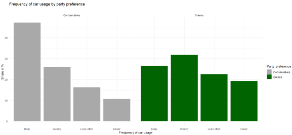
In this example, you clearly see that Conservative voters more often use their car “daily” whereas Green voters are more likely to rarely or “never” use a car.

This is a correlation in observational data. But is it also reflecting a causal relationship? For all that we know, voters of Green parties are often urban, well-educated people whereas Conservative voters are more likely to live in rural areas. For various reasons, thus, we can assume that place of residence (urban/rural) affects voting preferences. On the other hand, living in an urban agglomeration is also associated with better access to public transport, meaning it is more likely that you can get to work by bus or tram or even by bike, as opposed to living in a rural area where there are larger commuting distances and fewer connections by bus or train between places. So we could argue that place of residence is a confounding factor that needs to be controlled here.

Let’s divide our survey results and group people into urban/rural place of residence:

Our (made up) survey results are much less clear about a causal effect from party preference on car usage when we control for place of residence. By “controlling for”, we here simply divide our total survey respondents into groups of rural vs. urban dwellers and carry out the analysis separately within these groups. Below we’ll also discuss other more sophisticated methods.

As the results show, Green voters who live in the countryside are similar to rural Conservative voters in terms of their car usage in this fictional example. Conversely, urban Conservatives also less frequently use their car compared with rural Conservatives. So here we have a spurious correlation that is actually due to a compositional effect: Because the city population hosts proportionally more Greens than Conservatives, the Greens are overall less likely to use their cars on a daily basis. Controlling for place of residence, this effect almost completely disappears.

Does that mean we can be absolutely sure that there is no direct causal effect here? In general, I would always refrain from using causal language in observational studies. You need to convince your audience that you have considered all important confounding variables, and that they are in fact confounding variables, apart from addressing the usual statistical issues (is your sample size large enough, etc.), and then you could come to the “tentative” conclusion that there does not “appear to be” a direct effect here.

To conclude, you always have to think about whether there might be factors that affect BOTH your X and Y of interest, and include them in an analysis – if you don’t have data from a randomized experiment (no control variables needed there usually) but rather from observational studies. How do you “include” them or “control” them other than the simple separate plotting we’ve done here? We’ll discuss that below.

Here is the code to create the fake data and plots shown above:

library(tidyverse)

d <- data.frame("Party_preference" = rep(c(rep("Conservatives", 4), rep("Greens", 4)),2),
                "Place_of_residence" = c(rep("City",8), rep("Countryside",8)),
                "Car_usage" = c(22,33,26,19,18,31,28,23,58,23,12,7,52,34,6,8),
                "Frequency" = rep(c("Daily", "Weekly", "Less often", "Never"),4),
                "Weight" = c(.30,.30,.30,.30,.75,.75,.75,.75,.70,.70,.70,.70,.25,.25,.25,.25))
d$Frequency <- factor(d$Frequency, levels = unique(d$Frequency))
d$Car_usage_weighted <- d$Car_usage*d$Weight

ggplot(d, aes(x=Frequency,y=Car_usage_weighted,fill=Party_preference)) + 
  geom_col() + theme_minimal() + 
  scale_fill_manual(values=c("darkgrey","darkgreen")) +
  xlab("Frequency of car usage") + ylab("Share in %") +
  ggtitle("Frequency of car usage by party preference",subtitle = "") +
  facet_wrap(~Party_preference)

ggplot(d, aes(x=Frequency,y=Car_usage,fill=Party_preference)) + 
  geom_col() + theme_minimal() + 
  scale_fill_manual(values=c("darkgrey","darkgreen")) +
  xlab("Frequency of car usage") + ylab("Share in %") +
  ggtitle("Frequency of car usage by party preference and place of residence",subtitle = "") +
  facet_wrap(~Party_preference+Place_of_residence)

Collider variables: Do NOT control for those

Let’s get back to our example of smoking and covid infections in hospital patients. Even though the example is made up, there have been similar findings in the past leading to confusion over, e.g., a possible beneficial effect of drug abuse on rare genetical diseases in young mothers.

Basically, what we have looks like this:

We want to know whether smoking affects your probability of catching Covid. But our data is from hospital patients, so we also control for the factor “hospitalisation” (hospitalisation is held constant at the level “true”, and there are no observations with hospitalisation == “false”). Now, we know that Covid can get you into the hospital, but we also know that heavy smoking causes diseases that need stationary treatment independent of Covid. Therefore you see arrows pointing from both X and Y to the collider variable. This means that smokers have a generally higher risk of being in a hospital as opposed to non-smokers per se, and this risk is largely due to factors other than Covid which, at the time of this made-up example, affects only a small share of patients in this hospital.

This means that, in a representative sample of the total population, symptomatic Covid infections might actually be more prevalent among smokers (or there might be no difference), but here in the hospital smokers are over-represented for other reasons such as lung cancer, deflating the share of Covid patients vis-à-vis the non-smokers who less often suffer from cancer and thus their share of Covid patients is relatively larger.

We can easily reproduce this with some simulated data. In the following code example, we assign smokers and non-smokers in the general population the exact same risk of being hospitalized due to Covid. Then we assign a higher risk of getting hospitalized for other reasons to the smokers:

set.seed(2022)
population <- data.frame(smoking = c(rep("smoker", 20000), rep("non_smoker", 80000)),
                         covid_hospitalisation = rbinom(100000,1,.005))
population$other_hospitalisation[population$smoking=="smoker"] <- rbinom(20000,1,.07)
population$other_hospitalisation[population$smoking=="non_smoker"] <- rbinom(80000,1,.05)

population$in_hospital <- population$covid_hospitalisation | population$other_hospitalisation

We assigned a 0.5% chance of being hospitalized due to Covid to all persons in the population, but we assigned a slightly larger chance (7%) of being hospitalized for other reasons to smokers as opposed to non-smokers (5%). Of course, whether these figures are realistic or not is not the point here. Let’s check that in the general population, both groups have an equal proportion of Covid hospitalisation:

t.test(covid_hospitalisation~smoking, population)

Which gives us:

We see that among both smokers and non-smokers, roughly 0.5% of the population are in a hospital due to Covid at this point in time, and the small difference is due to random chance and not statistically significant given the p-value of 0.89.

Now let’s limit the data to all hospital patients and compare Covid rates among smokers and non-smokers:

hospital <- population[which(population$in_hospital),]
t.test(covid_hospitalisation~smoking, hospital)

Result:

Here we see that the non-smokers have a higher proportion of Covid patients (9%) as opposed to the smokers (6.5%), and this difference is statistically significant (p < .01). Which shows exactly our point here: Limiting the data to hospital patients results in a biased comparison of smokers and non-smokers which is not reflective of the true causal effect (which is zero in our example). In a real-world scenario, researchers often only have data from hospital patients and do not know the true effect in the general population. Which is why they need to consider potential collider effects in order to avoid to come to conclusions that are plain wrong.

To summarize: Whenever you have a variable that is affected by both X and Y, you need to leave it out of the equation. If you can’t do that (because, as in the example, the data were collected in a hospital and you don’t have any non-hospitalized participants), this means you need to interpret the data with caution and maybe refrain from making this kind of comparison at all.

Mediator variables (a.k.a. mechanisms)

Let’s assume that households with children have on average a lower household income as opposed to childless couples. One of the obvious reasons for this correlation is given by the fact that mothers or fathers often reduce their working hours to work part-time (or take maternal/paternal leaves) while their children are still young. Working less of course translates into a lower household income. Let’s look at the consequences in another (made-up) example dataset:

In this dataset, there is a clear negative correlation between the number of children in a household and the monthly income. Let’s assume other factors such as the number of adults living in the household are held constant.

If you want to replicate this, here is the (fake) replication data and code for the above plot:

set.seed(2022)
x = c(rep(0,1000),rep(1,500),rep(2,600),rep(3,300),rep(4,100))
m = rexp(2500,.2) *(-1) + 40
f = c(rexp(1000,.2) *(-1) + 40,rnorm(500,31,9),rnorm(600,30,10),rnorm(300,28,7),rnorm(100,25,5))
e = f* rnorm(2500,100,25)
d = data.frame(x,m,f,e)

ggplot(d, aes(x=factor(x),y=e)) + geom_boxplot() + theme_minimal() + ylim(0,8000) +
  xlab("Number of children <6 year old") + ylab("Household income in Euro") +
  ggtitle("Monthly income by number of children") +
  geom_smooth(method='lm',aes(group=1)) 

Now, let’s factor in the working time, broadly distinguishing between full-time and part-time workers:

Code for the plots:

ggplot(d[d$f>=35,], aes(x=factor(x),y=e)) + geom_boxplot() + theme_minimal() + ylim(0,8000) +
  xlab("Number of children <6 year old") + ylab("Household income in Euro") +
  ggtitle("Monthly income by number of children",subtitle = "only full-time (35+ hours/week)") +
  geom_smooth(method='lm',aes(group=1)) 

ggplot(d[d$f<=20,], aes(x=factor(x),y=e)) + geom_boxplot() + theme_minimal() + ylim(0,4000) +
  xlab("Number of children <6 year old") + ylab("Household income in Euro") +
  ggtitle("Monthly income by number of children",subtitle = "only part-time (<= 50%)") +
  geom_smooth(method='lm',aes(group=1)) 

Two things are to be noted about these two graphs: For once, if you look at the scales of the y axis, it is obvious that part-time workers earn less as opposed to full-time workers. And, interestingly, the association between the number of children and the income is not negative in neither of the two groups; if anything, it is positive, such that persons with more children earn on average just as much (or even a bit more) as opposed to childless persons – if they work the same amount of hours, that is.

Now what did we find here? Controlling for the number of working hours, having small children in the household does apparently not lead to less earnings (in this made-up example). Rather, our variable “working hours” fully explains why households with small children earn less compared with childless couples.

Importantly, this is a different case conceptually as opposed to the confounder example above about car usage among Green party voters. We did not reveal a correlation to be actually spurious here; rather, we found the reason for why X affects Y. But we have little doubt that X does in fact cause Y. Because the reduced working hours can plausibly be traced back to the small children in the household. As a DAG, this looks like the following:

Having children in the household affects your working hours, which in turn affects your household income. So “working hours” is one of (or maybe the only) causal pathway connecting X and Y. That is why it is called a mediator, or also called mechanism. It explains why X affects Y.

Again: Saying that children in the household doesn’t actually affect your household income, because the effect disappears when you control for working hours, would be wrong – X does affect Y via the mediator variable. There is for sure a total causal effect, there just does not appear to be a direct causal effect anymore when you consider working hours as a mechanism (see our boxplots above), which is why in the DAG above we could remove the direct arrow from children on income.

By contrast, in the vaccination example, if we control for the confounders (age etc.) and find no direct effect anymore, then we would say that there is in fact apparently no causal effect from X on Y.

Mediators can be controlled for (e.g., added to a regression model) if you want to assess what part of the effect can be attributed to the mechanism. But it makes sense to also provide a model without the mediators to see how large the total effect (direct + indirect effects) is.

Example: If you run a regression with the above data – summary(lm(e~x,d)) – you will find that an additional child lowers your income on average by 261 Euros, and this effect is statistically significant. If you add working hours to the equation – summary(lm(e~x + f,d)) – the effect will disappear. Using the stargazer package to export the regression models, a regression table could look like this:

Showing both models with and without the mediator variable lets you (and your audience) quickly recognize that, first, having children is in general associated with lower income, and, second, the effect is caused by parents working fewer hours. We’ll explain in greater detail what is going on in a multivariate regression in a bit.

What is a moderator variable?

A moderator is a variable that, if present, alters the effect of X on Y. Here are two examples to illustrate what that means:

• Having young children in the household leads to reduced working hours, as we saw above. But: Upon closer examination, we might find that females are much more likely to work part-time if small children are present whereas males most often continue to work full-time. This would mean that gender is a moderator to the effect of children (X) on working time (Y): If gender == female, the effect is large, but if gender == male, the effect is small.
• Your company is selling bottled beverages in four different countries. You are tasked with assessing whether changing the bottle material from plastic to glass (X) would result in increased sales (Y). So you’re trying a little experiment: You’re randomly picking a couple of stores across all four countries and ship glass bottles to these stores wheras all other stores are still receiving plastic bottles. In the subsequent months, you notice that sales development is indeed better in the stores that sold glass bottles. But: You also notice that the increase can be attributed to the stores in Germany and the Netherlands, wheres in France and Belgium, there was no significant difference between plastic and glass (again, I’m just making this up). Here, “country” moderates the effect of material on sales. In some countries, there is an effect, in others, there isn’t.

In other words, a moderator is responsible for a heterogenous treatment effect: The treatment (change in material) does not cause sales to increase across the entire treatment group; rather, there are sub-groups where the increase is significant, and others where it does not happen.

We can visualize a moderator effect as follows:

From the diagram, you can see the differences between a moderator variable and a mediator or confounder: A moderator variable has no causal connection to X whatsoever. We randomly selected stores in all countries, so “country” didn’t impact “material”. Conversely, “material” obviously can’t affect “country”. By contrast, a mediator is affected by X and a confounder affects X.

Similarly, having young children affects people’s working hours, and female gender moderates this effect: One’s gender does not change after having children, so it cannot be a mediator. Neither can gender have an effect on whether or not you have children, so it’s not a confounder (leaving aside the possibility that more children might live in single-mother households). But gender does play a role in determining the effect size.

So by the rules introduced in the beginning of this article, moderator variables are not a necessity to include when assessing the correlation of two variables. Leaving it out does not bias the results, as would happen if you fail to adjust for a confounding variable. You simply gain more insight into the black box if you consider the moderator: You realize that your data are heterogeneous and that for some sub-groups in your data, the treatment works differently compared with other sub-groups. This is important, e.g., when assessing the efficacy of a drug in treating an illness, where the effect may vary by factors such as pre-existing conditions, other medication, or genetic factors.

If you theoretically suspect that there might be heterogeneous treatment effects and you want to assess whether there is a moderator present, you can do so, again, either by simply filtering the data to e.g. males or females only and then see if you get different statistics in these sub-groups. If you have multiple variables and a more complex model, you can include an interaction effect into a regression or ANOVA to see if there is a moderator effect (e.g., gender * working hours). We won’t go into the details about interaction effects here, but let’s have a look at how you can generally “control for” variables, with a special focus on regression and matching.

How do I “control”/”adjust” for variables in R?

Quick summary of what we have discussed so far:

• If you have data from a randomized experiment, you likely do not need to worry about confounders, colliders etc.
• If you have observational data, by contrast, start your analysis by drawing a diagram of the hypothesized influences between your variables of interest (X and Y) as well as other potentially relevant variables.
• Variables that point to both X and Y are confounders that must be controlled for in the analysis. Failing to do so will result in biased statistical results.
• Mechanisms (X affects M affects Y) can be included if you want to shed light on what part of the effect of X on Y is mediated by M, but the total effect of X on Y is given by an analysis without M, so make sure to present at least one statistic where you leave the mechanisms out.
• Other types of variables are at best unnecessary, at worst inducing new bias (through collider variables), so leave them out.

So how do you “control for” or (synonyms) “adjust for” / “hold constant” confounding variables? Here are three widely employed strategies, from most simple to a bit more complex.

Option 1: Partition data into sub-groups

This is the most easy way to go and almost self-explanatory. See the graphs and code for the example of car usage among Green party voters above. If you want to make sure that a confounding variable isn’t biasing your results, you simply filter your data such that the confounding variable is constant in the sub-set.

This option is viable if you have a small number of confounders (i.e. only one or two) and these variables have only a few distinct values.

Examples:

• Your theoretical model suggests that gender is the only confounding variable. So you simply divide the data into subsets for males and females and re-run the analysis (e.g., a barchart, a statistical test such as a t-test or a correlation) in each of the two subsets separately.
• In the example of vaccines and mortality rates, you want to rule out the possibility of age as a confounder. Therefore, you filter the data to only, say, people aged 30 to 39, and then compare death rates by vaccination status. Repeat with age group 40 to 49, and so on.

In the second example, you can see that this approach is already a bit problematic since you have to present many statistics (otherwise you would appear to be cherry-picking if you only show the results for two age groups), and, if you define the age bracket too broadly (e.g. “60 years and older”), you might not have really held your confounder constant and there might still be differences in X and Y by age within your sub-group, but then if you make the bracket too narrow (e.g. only 60 to 62 year-olds), your sample size probably gets small. Similar problems arise if you have multiple confounders; e.g., you expect that gender, education and also country of birth are important variables to control, so the approach of filtering the data and creating subsets gets more and more tedious and your sample sizes decrease (e.g., foreign-born females with low education, native-born males with intermediate education, etc.). Therefore, in case of several and/or continuous confounders, most researchers resort to some form of multivariate regression.

Option 2: Multivariate regression

I can’t give a comprehensive introduction into regression analysis here; I assume you have heard of the basics elsewhere. But I’ll try to explain in simple terms what “controlling for” a third variable in a regression model means, because in my experience, this is often poorly understood.

Let’s look at a new example: Assume we have a study among school children aged 6 to 17 and we want to assess whether there is an effect of exercising on the resting heart rate. In general, we assume that the more you exercise (X), the slower your pulse at rest (Y) will be. But: We suspect that age is a confounding factor here, because we assume that older children have more gym classes and sports club memberships as opposed to younger children, and we also know that the average resting heart rate decreases by age from around 85 bpm among 6 year-olds to around 73 bpm among 17 year-olds. Thus, age is a confounding factor here; it affects both our X and Y of interest.

We therefore need to control for age, otherwise there is a risk of finding a correlation that is actually spurious: We might find that children who exercise more have lower resting heart rates, but that might just be because older children exercise more and also for biological reasons have slower heart rates. Of course we might consider additional factors, such as, e.g. obesity, but let’s keep it simple.

Here are some fake data for your replication:

set.seed(2022)
age <- sample(6:17, 200, T)
exercise <- abs(2*(age/max(age) + rnorm(200,0,1))+1)
heart_rate <- 85+(6*12/11) - age*(12/11) - exercise/max(exercise)*0.8 + rnorm(200,0,5)
dat <- data.frame(age, exercise, heart_rate)

ggplot(dat, aes(x=exercise, y=heart_rate)) + 
  geom_point() + 
  geom_smooth(method="lm") +
  theme_classic() + ggtitle("Resting heart rate by physical activity among school children") +
  xlab("Exercise (hours/week)") + ylab("Resting heart rate (bpm)")

This gives us this plot with a regression line:

We see that among the 200 children in our dataset, there is a negative correlation between exercising and the heart rate at rest. Those who never exercise have on average a heart rate above 80 bpm, while those that exercise 5 hours per week have on average around 75 bpm. The correlation is not very strong, which is apparent by the large spread of the points over the plot area; there are many children who exercise a lot but still have a high heart rate, and vice versa. However, there is a visible correlation.

We can formally test the correlation and also run a first (bivariate) regression model. Note that we deliberately disregard our confounding factor “age” at this stage in order to see how it affects our results when we do take age into account.

cor.test(dat$exercise, dat$heart_rate)
summary(lm(heart_rate ~ exercise, dat))

Which gives us:

We see that exercising and heart rate at rest are correlated with r = -0.35, which is a negative correlation of moderate strength. The result is also statistically significant (p value < 0.001), which means that if the true correlation (among all school children in our population) was zero, it would be very unlikely to obtain a result like this (or more extreme) in a sample of 200 children. Thus, if our sample of children is representative of the total population (the significance test does not tell us this of course), we can be quite sure that there is in fact a negative correlation between these variables that cannot be explained by random chance. The regression output tells us that a child with 0 hours of exercising per week has on average a heart rate of 82 bpm (= the intercept), and with every hour of additional exercise, this rate decreases by 1.27 bpm.

So far, this would be the standard way to do a regression if there were no confounding variables. But, since we have strong reasons to believe that age might distort our analysis here, we should control for age in this analysis. How do we do this? In R, we simply add age to the equation. But what does that mean? Instead of a regression line (see plot above), we now have a three-dimensional model (exercise, age, and heart rate). So the regression line becomes a regression plane (or surface). This is how this looks like with our data:

summary(lm(heart_rate ~ exercise + age, dat))

library(rsm)
mod <- rsm(heart_rate ~ exercise + age, dat)
persp(mod, form = ~ exercise + age, 
      zlab = "Heart rate at rest", main = "Heart rate as a function of exercise and age")

The first line of code gives us the regression model controlling for age, the rest shows the regression plane:

Let’s start with the 3D graph since this is the easiest way to understand what’s going on. (Note that in published papers, you rarely see this kind of graphical representation, simply because usually more than one control variable is considered and then you would need 4, 5, or more dimensions to plot the results, which is of course not possible; but for didactical reasons I think this is a good way to understand the model).

You can easily see here that the resting heart rate not only depends on exercising, but even stronger on age among the children in our sample. If you look at the left “wall” of the cube, you see the steep increase in heart rate the younger the child gets. For us, the interesting part is whether the effect of exercise is still there once age is also present in the model. Indeed, we see that the plane is weighed down to the right, indicating that the more a child exercises, the lower the heart rate. You can see this is the case for older as well as for younger children: Among children aged 6, the model predicts values between 85 bpm (no exercise) to 80 bpm (8 hours exercise a week). Among children aged 17, whose heart rate is generally lower, exercising has a similar effect, bringing down the heart rate at rest from around 74 bpm (no exercise) to less than 70 bpm (8 hours exercise per week).

Note that the standard regression model we are running here is a linear model, which means it by default assumes linear relationships between all variables. This is important because the model as is could not inform us about so-called heterogeneous treatment effects. The latter could mean that among 17 year olds, exercising has a bigger effect on the heart rate as opposed to 6 year olds where it hardly makes any difference. This kind of finding cannot be produced by our code above. You could reveal patterns like this with interaction terms or non-linear approaches (simple approach: dummy variables for different age groups and interact each with exercise; resulting in an equation such as heart_rate ~ exercise*age_6to9 + exercise*age_10to12 etc.). In many cases, however, the standard linear model works just fine.

As you can see, our analysis shows that exercising has an effect on the resting heart rate over and above what the correlations between age and exercising as well as age and heart rate can explain. This is an example where the bivariate correlation is not (entirely) spurious, it still exists even after controlling for age. This is what we wanted to confirm with the analysis.

If you, however, take a look at the regression output above, and compare it with the model without age, you will note that the effect of exercise has become weaker. Previously, we estimated that with every hour of exercise, your resting heart rate would decrease by 1.27 beats per minute. But this estimate was biased because we did not control for age as a crucial confounding variable. Doing so gives us an estimate of -0.55, meaning that one hour of exercise decreases your heart rate by 0.5 bpm. This is still statistically significant. It can be interpreted as the effect from one hour of exercising per week on the heart rate at rest for children at an average age (in our sample).

Thus, we found out that controlling for age results in a smaller effect of exercising on the heart rate, but the effect is still there and is still statistically significant. In the example of car usage by green party affiliation, we found that our main effect completely disappeared once adjusting for a confounding variable. In the example of deaths after vaccination, it is likely that an adjusted model would even yield an effect that goes in the opposite direction of the original reported correlation.

So you see: Not controlling for a confounder variable can result in severe bias; your bivariate correlation could still be there after adjusting for the confounder, or it might disappear, or it might even reverse. It is thus absolutely crucial to, before carrying out an analysis with observational data, really think about the relations between your variables and possible distortions due to confounding variables. Imagine the damage done by business decisions, or medical decisions, or political actions, that are based on biased statistical analyses, poorly understood by decision makers who are not trained in basic statistics.

Final remark about regression: There are of course many variants and advancements over the standard linear model which can help you identify causal effects (or tentatively claim that you might have identified them) when you have special data structures. For instance, if you have longitudinal data of multiple individuals (or countries, etc.), also known as time-series cross-sectional or panel data, there are special regression models that can make use of both the temporal and the inter-individual variation. I might write a post about panel regression models in R in the future. Or, if you are less concerned with identifying the causal effect of X, but more interested in predicting the outcome Y (e.g., which individuals will develop severe Covid illness based on a multitude of clinical characteristics), models other than regression are often better-suited since they can overcome a number of limitations to regression (e.g., multi-collinearity, see below). Examples include machine-learning algorithms such as random forests. I might make a post about those too. Either way, I hope by now you understand the general idea behind “controlling variables” in order to identify causal effects; we’ll finish with another way to do that.

Option 3: Propensity-score matching

The two options above are the most prevalent methods in most applied research. Let’s finish this article with an approach which is less known but is also worth considering in some situations.

Let’s quickly explain one of the main reasons for why many regression analyses in applied research are problematic: The linear regression model assumes that the predictor variables are uncorrelated. In our examples above, the predictors are never uncorrelated. That’s the whole point of including a control variable in the analysis, because we assumed that, e.g., exercising and age are somewhat associated and thus leaving out age would result in distorted results. Ignoring the assumption of uncorrelated predictors is often fine, but when this so-called multicollinearity reaches high levels, your results will be unstable and will be highly impacted by unusual outliers in your data (e.g., one older kid who exercises a lot but has, for some reasons that you don’t take into account in your model, a very high heart rate at rest). Philip Schrodt lists disregarding collinearity as the first of his “seven deadly sins” of applied regression research.

An example: In a respected German weekly newspaper, I read an article on overpopulation and climate change (the article was also re-printed on the German federal agency for political education’s website). A sub-heading of the article reads: “Overpopulation will not be a problem in the long run”. With regard to the effect of human population growth on the environment, the article contains the following statement: “In places where the population grows, […] less [CO2] is being emitted.” So the article basically says: Population growth is not a problem for the environment; in fact, population growth is correlated with less CO2 emissions, so “overpopulation” will not be a problem. If anything, high fertility rates will help fighting climate change!

If you have read the rest of this post, I hope your alarm bells are ringing if you read a statement like this. This is a prime example of a spurious correlation, caused by omitted variable bias (i.e. no adjustment for crucial confounding variables). Again, we won’t go into the substantial details regarding the topic (population growth and climate change); it suffices to say that it is well known that both the fertility rate as well as the rate of CO2 emissions of a country are heavily affected by the level of socio-economic development, as measured by factors such as income, urbanization, or industrialization. As in our other examples above, we need to control for this (and probably other) confounding factors, but here the methodological problem of collinearity is very acute and our standard aproaches such as linear regression are therefore error-prone.

Especially when you’re dealing with aggregate data on the level of countries from all over the world, you often have very strong levels of collinearity between various variables that researchers like to put into their models as “control variables”, such as per-capita income, education, urbanization, democracy, geography, as well as various other demographic, historical, ethno-cultural and other factors. The problem is: Some countries such as Norway, New Zealand, or Canada have high income levels, high per-capita CO2 emissions, and low fertility rates. Other countries such as Afghanistan, Somalia, or Haiti have low income levels, low per-capita CO2 emissions, and high fertility rates. So these variables are all highly correlated.

Which causes the following issue: There are hardly any countries that have high income levels but low CO2 emissions, or low income and also low fertility rates. These kinds of countries simply don’t exist, except for maybe some rare special cases. But we would need this kind of variation in order to properly perform a multivariate regression! Think about the previous example, if all older kids with lower heart rates were working out, wheres all younger kids with higher heart rates were never exercising, then how could we have arrived at the regression plane in the figure in the previous section? Because most parts of the surface would be void of any actual data points.

In fact, with perfect collinearity, a multivariate regression simply does not work and your software would automatically omit at least one of the variables and give you a warning. But in real life, collinearity is mostly not perfect, so the software does not give you any warning and is technically able to perform the analysis even though the results must be interpreted with extreme caution. Example: A few small Arabic emirates have high income levels and also above-average fertility, wheras most other countries in the world have either high income and low fertility rates or vice versa. If this is the case, then the small number of special cases technically “save” the analysis, making collinearity less than perfect, but as a result this handful of countries have a very high impact on your results.

One method to alleviate this problem is given by propensity-score matching. Matching means that you don’t use all your data, but you try to find, for your selected group of “treatment” units, counterparts that are most similar in all other regards except for the treatment. An example to explain this:

• A vaccine study wants to know whether adverse effects after vaccination (e.g., myocarditis) can be causally attributed to the vaccine. They have a sample of persons from different age groups who recently have received a vaccine. For each of these persons, they are looking for a statistical twin, i.e. an otherwise similar but unvaccinated person. So they seek to match a 65 year old woman with diabetes who has recently been vaccinated to a 65 year old woman with diabetes who has not been vaccinated, and so on.
  This gives them a control group that can meaningfully be compared to the treatment group. They can then compare the rate of myocarditis cases in both groups and thereby estimate the treatment effect from vaccination. In their full sample, they probably have many old people with pre-existing conditions that have been vaccinated but much fewer unvaccinated old people with pre-existing conditions; and vaccination, age, co-morbidities, as well as other factors are all correlated so a linear regression model might give biased results. Filtering the data to the matched couples cleans the data of data points that have no substantial information value and allows for a more intuitive interpretation.

Let’s look at how you can perform propensity-score matching with some simulated data about the relationship between population growth and climate change introduced above.

I’m simulating fake data instead of downloading real data so that you can quickly reproduce the analysis, but also for another reason: I can specify the “true” causal relation in the data and then see whether our models such as correlation or matching are actually giving us good estimates of the true relations.

set.seed(2022)
dat <- data.frame(gdp_cap = rexp(200,0.0001)**(.8)*20)
dat$fertility <- (dat$gdp_cap/max(dat$gdp_cap))**(1/10)*-10+11 + rnorm(200,0,.6)
dat$urban <- dat$gdp_cap/max(dat$gdp_cap) * .7 + dat$fertility/max(dat$fertility) * -.7 + rnorm(200,0,.5)
dat$urban <- dat$urban - min(dat$urban)
dat$urban <- dat$urban/max(dat$urban)
dat$co2 <- dat$gdp_cap/max(dat$gdp_cap) * 600 + dat$fertility/max(dat$fertility) * 300 + rnorm(200,0,10)

In the last line, I specify here that the CO2 emissions of a country are positively affected by both the per-capita wealth as well as the fertility. Thus I’m saying higher fertility rates (and thus more population growth, causing more urban sprawl, more cars, etc.) translates to increased CO2 emissions. Again, let’s not discuss the actual state of the research on this topic; here it is only important that I created the data in a way that fertility levels have a positive effect on CO2 emissions. But CO2 emissions depend even more strongly on the income level (GDP per capita) of a country in our simulation. And the income level, in turn, has a negative effect on fertility in our code above.

Let’s look at a correlation matrix of all the indicators in the dataset:

cor(dat)

You can see that there is a strong positive correlation between GDP and CO2 emissions, and there is a strong negative relation between GDP and fertility. And now the interesting part: There is a negative correlation between fertility and CO2. Meaning that Countries with higher fertility rates emitt less CO2, just as the German newspaper article was saying. But how can that possibly be the case, when we have designed the data such that fertility positively affects CO2 emissions? The reason for that is the high collinearity between GDP and fertility, causing most high-income countries that emitt a lot of CO2 to have low fertility rates. So it looks like fertility rates are negatively correlated with CO2, although the true causal effect is positive.

Let’s try a matching procedure with this data. The package used as well as some explanations about matching can be found in this paper.

library(MatchIt)
dat$fertility_below_2 <- ifelse(dat$fertility <= 2,1,0)
set.seed(2022)
m1 <- matchit(fertility_below_2 ~ gdp_cap + urban, data=dat, method="nearest", distance="glm")
summary(m1)
plot(m1, type="jitter", interactive = F)

We first dichotomize our “treatment”, i.e. we need to create two groups which we (arbitrarily) define by whether or not a country has a total fertility rate of fewer than 2 children. Then we perform the matching, searching for the nearest neighbor for every country in the low-fertility group among the countries in the high-fertility group. We use GDP per capita and urbanisation as the characteristics that should be as similar as possible among our statistical twins. This gives us the following output:

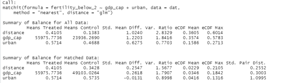
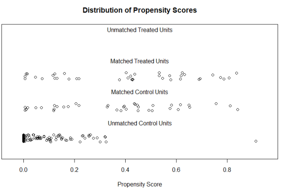
You can see that initially, our groups were very dissimilar: The low-fertility countries had income levels more than twice as high as compared with the high-fertility countries. After matching, the balance is still not perfect, but the differences were greatly reduced (56,000 € vs. 49,000 € per capita). The urbanization rate is now equal (57% vs. 57%) in both groups whereas there previously was a 10% difference. So our two groups can now be compared more meaningfully than before. The plot shows that many observations were disregarded by the matching algorithm, these are the countries that have high fertility rates, are very poor, and are thus not very informative for our analysis.

In a real-world application you might want to aim at getting an even better balance, i.e. even more similar values for GDP post-matching (or take the log of GDP beforehand…). But let’s continue and see what we can do with our matched data:

mdat <- match.data(m1)

ggplot(mdat, aes(x=factor(fertility_below_2), y=co2)) + geom_boxplot() + geom_jitter(width=.1) +
  stat_summary(fun.y = "mean", geom = "point", pch="-", size=20, colour = "red") +
  ylab("CO2 emissions in t") +
  theme_minimal() + scale_x_discrete(name="Fertility rate", labels=c("more than 2 children", "fewer than 2 children"))  
t.test(co2 ~ fertility_below_2, mdat)

After creating the matched dataset, you can plot the two groups, perform a difference-in-means test, or run a regression (where you could still include e.g. GDP since it was not perfectly neutralized by the matching). The above code gives us:

Now we obtain that – once income and urbanization levels have been held at comparable values – countries with a lower fertility rate actually have lower CO2 emissions. The difference is not statistically significant (we’re down to 76 observations at this point), but we now have at least an estimate that points into the correct direction. Whereas the naive, bivariate correlation would suggest that countries with a high fertility rate emitt less CO2, when using a method that allows for a (tentatively) more causal interpretation, we find that if anything, the opposite is true.

Note that matching is no perfect cure for multi-collinearity, you still need some degree of “overlap” of the distributions (i.e. not all poor countries should have high fertility and vice versa), otherwise you don’t find any matching partners except for, again, the unusual outliers. But in many cases matching makes sense, not least because the results can easily be interpreted and also explained to decision makers (Instead of saying: “Here is a regression table with 14 variables, from the p-value of the fourth entry from the top left you can see that our drug does not work”, you can say: “Here is a barchart comparing people who took the drug with their statistical twins (in terms of age, gender, etc.), who didn’t take the drug. Note that the bars are of equal height, our drug does not work”).

The end

If you made it through this whole article, then thank you for reading and I hope it was of help. PS: I previously used a few of the examples in this article in statistics classes, so if you think the examples might be helpful for your courses as well, or if you’re a student and want to use the code or plots in a presentation, feel free to use it. A link to this page would be appreciated, if you want to include a source in a footnote or so.