
Easy Interpretations of ADF Test in R
[This article was first published on K & L Fintech Modeling, and kindly contributed to R-bloggers]. (You can report issue about the content on this page here)
Want to share your content on R-bloggers? click here if you have a blog, or here if you don't.
This post shows how to interpret the results of the augmented Dickey-Fuller (ADF) test easily with the help of Hank Roark’s R function. His R function provides kind descriptions of the results of a unit root ADF test. I explains why this description is consistent with the ADF hypothesis test. Want to share your content on R-bloggers? click here if you have a blog, or here if you don't.
Easy Interpretations of ADF Test
The purpose of this and previous post are to be familiar with the ADF test.
In the previous post below, we have implemented ADF test for a unit root by using ur.df() function in urca R library.
In particular, we have encountered the some case where there may or may not be either trend or drift or both. In addition, it is a little time-consuming to interpret the results of the ADF test. Fortunately, Hank Roark provides a R function which generates the description of the ADF test result. Owing to this convenient R function, we can easily summarize the output of ADF test and save our time.
We use the same data as in the previous post and perform the ADF test whether the LRY time series contains a unit root or not.
Hank Roark’s R function
Hank Roark’s R function can be found at https://gist.github.com/hankroark/968fc28b767f1e43b5a33b151b771bf9. I just added three lines to dislpay the formula of model.
############################################################################ # This R function helps to interpret the output of the urca::ur.df function. # The rules are based on https://stats.stackexchange.com/questions/ # 24072/interpreting-rs-ur-df-dickey-fuller-unit-root-test-results # # urdf is the output of the urca::ur.df function # level is one of c(“1pct”, “5pct”, “10pct”) # # Author: Hank Roark # Date: October 2019 ############################################################################ interp_urdf <– function(urdf, level=“5pct”) { # urdf = lt.adf.df.trend$LRY # level = “5pct” if(class(urdf) != “ur.df”) stop(‘parameter is not of class ur.df from urca package’) if(!(level %in% c(“1pct”, “5pct”, “10pct”) ) ) stop(‘parameter level is not one of 1pct, 5pct, or 10pct’) #cat(“========================================================================\n”) cat( paste(“At the”, level, “level:\n”) ) if(urdf@model == “none”) { cat(“The model is of type none : “); print(urdf@testreg$call$formula) tau1_crit = urdf@cval[“tau1”,level] tau1_teststat = urdf@teststat[“statistic”,“tau1”] tau1_teststat_wi_crit = tau1_teststat > tau1_crit if(tau1_teststat_wi_crit) { cat(“tau1: The null hypothesis is not rejected, unit root is present\n”) } else { cat(“tau1: The null hypothesis is rejected, unit root is not present\n”) } } else if(urdf@model == “drift”) { #cat(“The model is of type drift\n”) cat(“The model is of type drift : “); print(urdf@testreg$call$formula) tau2_crit = urdf@cval[“tau2”,level] tau2_teststat = urdf@teststat[“statistic”,“tau2”] tau2_teststat_wi_crit = tau2_teststat > tau2_crit phi1_crit = urdf@cval[“phi1”,level] phi1_teststat = urdf@teststat[“statistic”,“phi1”] phi1_teststat_wi_crit = phi1_teststat < phi1_crit if(tau2_teststat_wi_crit) { # Unit root present branch cat(“tau2: The first null hypothesis is not rejected, unit root is present\n”) if(phi1_teststat_wi_crit) { cat(“phi1: The second null hypothesis is not rejected, unit root is present\n”) cat(” and there is no drift.\n”) } else { cat(“phi1: The second null hypothesis is rejected, unit root is present\n”) cat(” and there is drift.\n”) } } else { # Unit root not present branch cat(“tau2: The first null hypothesis is rejected, unit root is not present\n”) if(phi1_teststat_wi_crit) { cat(“phi1: The second null hypothesis is not rejected, unit root is present\n”) cat(” and there is no drift.\n”) warning(“This is inconsistent with the first null hypothesis.”) } else { cat(“phi1: The second null hypothesis is rejected, unit root is not present\n”) cat(” and there is drift.\n”) } } } else if(urdf@model == “trend”) { #cat(“The model is of type trend\n”) cat(“The model is of type trend : “); print(urdf@testreg$call$formula) tau3_crit = urdf@cval[“tau3”,level] tau3_teststat = urdf@teststat[“statistic”,“tau3”] tau3_teststat_wi_crit = tau3_teststat > tau3_crit phi2_crit = urdf@cval[“phi2”,level] phi2_teststat = urdf@teststat[“statistic”,“phi2”] phi2_teststat_wi_crit = phi2_teststat < phi2_crit phi3_crit = urdf@cval[“phi3”,level] phi3_teststat = urdf@teststat[“statistic”,“phi3”] phi3_teststat_wi_crit = phi3_teststat < phi3_crit if(tau3_teststat_wi_crit) { # First null hypothesis is not rejected, Unit root present branch cat(“tau3: The first null hypothesis is not rejected, unit root is present\n”) if(phi3_teststat_wi_crit) { # Second null hypothesis is not rejected cat(“phi3: The second null hypothesis is not rejected, unit root is present\n”) cat(” and there is no trend\n”) if(phi2_teststat_wi_crit) { # Third null hypothesis is not rejected # a0-drift = gamma = a2-trend = 0 cat(“phi2: The third null hypothesis is not rejected, unit root is present\n”) cat(” there is no trend, and there is no drift\n”) } else { # Third null hypothesis is rejected cat(“phi2: The third null hypothesis is rejected, unit root is present\n”) cat(” there is no trend, and there is drift\n”) } } else { # Second null hypothesis is rejected cat(“phi3: The second null hypothesis is rejected, unit root is present\n”) cat(” and there is trend\n”) if(phi2_teststat_wi_crit) { # Third null hypothesis is not rejected # a0-drift = gamma = a2-trend = 0 cat(“phi2: The third null hypothesis is not rejected, unit root is present\n”) cat(” there is no trend, and there is no drift\n”) warning(“This is inconsistent with the second null hypothesis.”) } else { # Third null hypothesis is rejected cat(“phi2: The third null hypothesis is rejected, unit root is present\n”) cat(” there is trend, and there may or may not be drift\n”) warning(“Presence of drift is inconclusive.”) } } } else { # First null hypothesis is rejected, Unit root not present branch cat(“tau3: The first null hypothesis is rejected, unit root is not present\n”) if(phi3_teststat_wi_crit) { cat(“phi3: The second null hypothesis is not rejected, unit root is present\n”) cat(” and there is no trend\n”) warning(“This is inconsistent with the first null hypothesis.”) if(phi2_teststat_wi_crit) { # Third null hypothesis is not rejected # a0-drift = gamma = a2-trend = 0 cat(“phi2: The third null hypothesis is not rejected, unit root is present\n”) cat(” there is no trend, and there is no drift\n”) warning(“This is inconsistent with the first null hypothesis.”) } else { # Third null hypothesis is rejected cat(“phi2: The third null hypothesis is rejected, unit root is not present\n”) cat(” there is no trend, and there is drift\n”) } } else { cat(“phi3: The second null hypothesis is rejected, unit root is not present\n”) cat(” and there may or may not be trend\n”) warning(“Presence of trend is inconclusive.”) if(phi2_teststat_wi_crit) { # Third null hypothesis is not rejected # a0-drift = gamma = a2-trend = 0 cat(“phi2: The third null hypothesis is not rejected, unit root is present\n”) cat(” there is no trend, and there is no drift\n”) warning(“This is inconsistent with the first and second null hypothesis.”) } else { # Third null hypothesis is rejected cat(“phi2: The third null hypothesis is rejected, unit root is not present\n”) cat(” there may or may not be trend, and there may or may not be drift\n”) warning(“Presence of trend and drift is inconclusive.”) } } } } else warning(‘urdf model type is not one of none, drift, or trend’) cat(“========================================================================\n”) } | cs |
R code
In the following R code, we perform ADF test for denmark time series by using ur.df() function and apply Hank Roark’s R function to these results.
#========================================================# # Quantitative ALM, Financial Econometrics & Derivatives # ML/DL using R, Python, Tensorflow by Sang-Heon Lee # # https://kiandlee.blogspot.com #——————————————————–# # Augmented Dickey-Fuller (ADF) Test with # easy interpretations using Hank Roark R function #========================================================# graphics.off() # clear all graphs rm(list = ls()) # remove all files from your workspace library(urca) # ur.df interp_urdf <– function(urdf, level=“5pct”) { # body of Hank Roark R function } #======================================================== # Data #======================================================== data(denmark) # lv data lv <– denmark[,c(“LRM”,“LRY”,“IBO”,“IDE”)] nr_lv <– nrow(lv) # 1st differenced data df <– as.data.frame(diff(as.matrix(lv), lag = 1)) colnames(df) <– c(“LRM”, “LRY”, “IBO”, “IDE”) #======================================================== # ADF test of level variables #======================================================== # Level adf.lv.n.LRY = ur.df(lv$LRY, type=‘none’ , selectlags = c(“BIC”)) adf.lv.d.LRY = ur.df(lv$LRY, type=‘drift’, selectlags = c(“BIC”)) adf.lv.t.LRY = ur.df(lv$LRY, type=‘trend’, selectlags = c(“BIC”)) # 1st difference adf.df.n.LRY = ur.df(df$LRY, type=‘none’ , selectlags = c(“BIC”)) adf.df.d.LRY = ur.df(df$LRY, type=‘drift’, selectlags = c(“BIC”)) adf.df.t.LRY = ur.df(df$LRY, type=‘trend’, selectlags = c(“BIC”)) #======================================================== # Automatic Interpretation by using Hank Roark procedure #======================================================== # Level interp_urdf(adf.lv.n.LRY, “5pct”) interp_urdf(adf.lv.d.LRY, “5pct”) interp_urdf(adf.lv.t.LRY, “5pct”) # 1st difference interp_urdf(adf.df.n.LRY, “5pct”) interp_urdf(adf.df.d.LRY, “5pct”) interp_urdf(adf.df.t.LRY, “5pct”) | cs |
Interpretation
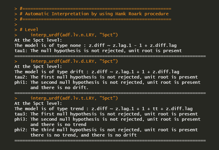
For the case of the LRY level variable, we have the following results which indicate the presence of a unit root. This is the same interpretations as in the previous post.
For the case of the LRY 1st diff. variable, we have the following results which indicate no unit root. This is also the same interpretations as in the previous post. In particular, this test displays some warning messages regarding the some inconclusive terms.
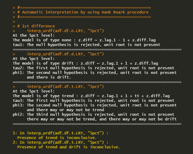
As can be seen in the previous post, logarithm of real income contains a unit root and can be stationary time series by differencing the first order.
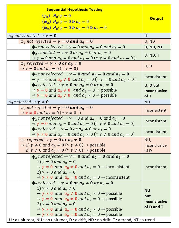
Structure of Hypothesis Testing
Now let’s understand the way Hank Roark’s R function deliver the output. I made the following summary table of the 3rd ADF regression model with a drift amd a trend for your better understanding.
Concluding Remarks
In this post, we use Hank Roark’s R function to get output descriptions of ADF test. Since this is easy to use, it can be applied to VAR or VECM or some machine learning models which requires stationarity of variables. \(\blacksquare\)
To leave a comment for the author, please follow the link and comment on their blog: K & L Fintech Modeling.
R-bloggers.com offers daily e-mail updates about R news and tutorials about learning R and many other topics. Click here if you're looking to post or find an R/data-science job.
Want to share your content on R-bloggers? click here if you have a blog, or here if you don't.