This tutorial might be for you if, e.g.:

• You have a lot of customer e-mails, or online-reviews on sales platforms or app stores for your product, etc., and you want to have a statistic based on the content of the texts: How many customers are complaining about a defect product vs. how many have a question about the functionality vs. how many give positive feedback about a certain feature, …
  So in the end you could have a statistic for management such as “complaints about defect products occured in 12% of all customer communictation this year, up from 8% last year”. Or you could also use the labels for further processing; e.g. all texts containing complaints are forwarded to the service division, all questions about spare parts are forwarded to sales, and so on. But you don’t want to read all 20,000 mails/reviews yourself; instead you want an algorithm to do (most of) the work.
• You are a scientist and want to classify tweets by, say, politicians according to which topics they write about on Twitter (foreign policy, taxes, migration, corona virus, etc.). You want to have statistics by, e.g., party affiliation or gender or regional background of the politicians, how these factors affect differences in Twitter topics. You could go on and use the results for, say, a cluster analysis to investigate whether, for example, Republicans from big US cities are more similar to Democrats in terms of what they tweet about as compared with Republicans from rural areas. And so on.

There are a lot of other different use cases, but I hope you get the idea. The technical term of what we are going to do is topic classification (or text classification). This is a sub-field of natural language processing (NLP) in machine learning. This method differs from other text mining techniques which are unsupervised machine learning methods. Unsupervised means that without any human input, an algorithm analyzes the provided text and outputs, e.g., clusters of texts based on their general similarity or topics (look into, e.g., topic modelling with latent dirichlet analysis, similar to principal component analysis (or factor analysis)).

Here, by contrast, we are using a supervised method. This means that the algorithm is not figuring out by itself what kind of topics your customers write about in their e-mails. Rather, you use a (sufficiently high) number of examples where you yourself tell the machine “this text is about topic A”, and “that text is about topic B”.

What you can vs. can’t do with this method

What are the pro’s and con’s of this approach? First off, a supervised model obviously requires more work as compared with an unsupervised method. Depending on the structure of the data and the number of topics you want to identify, you might need to read hundreds of texts yourself and manually assign them to the topics you want the machine to learn (or you can outsource this to, e.g., Amazon Mechanical Turk). In addition, the manual assignment of topics might not be undisputed. Another person might have annotated the data in a different way as compared to you (or the crowd workers who did it). Another limitation is that, if you train the algorithm to recognize five distinct topics, it will only ever recognize these five topics and will have no means to notify you if “new” topics are coming up. For instance, if you train a supervised topic classification algorithm to detect complaints about the weight, the color, and the battery lifetime of your product in reviews on Amazon, but at some point in the future there is a surge in customers complaining about transport damages, your algorithm will not identify this problem.

The advantage of training an algorithm on a pre-determined number of topics, on the other hand, is that these models can usually achieve a high accuracy if given a sufficiently large number of training examples. Most highly effective AI algorithms rely on human-annotated training data. For instance, image-recognition algorithms in computer vision often use images annotated by internet users (think Google captchas) as training data. By contrast, unsupervised methods like topic modeling often give results that require some additional interpretation (the algorithm does not name the topics it allocated for you), and they are sensitive to model parameters such as the number of topics to be extracted. So if you already know what you are looking for in your texts in terms of topics, the approach presented here will work for you. If you want an algorithm to be able to detect new and unseen patterns, or if you don’t have time or money to generate human-annotated training data, you will have to look into other methods.

Summary: The 8 steps of supervised topic classification

In short, we will proceed as follows:

1. Get data.
2. Create a random sample of the total dataset (e.g., 1,000 out of 20,000 texts) which we use for training and testing the algorithm.
3. Manually go through this sub-samle of the data and assign texts to one or more topics, like in the example below.
4. Divide your manually labelled data into training (e.g., 700 texts) and testing (e.g., 300 texts) datasets.
5. Train algorithms using out-of-the-box models provided in R packages or through web API’s (e.g., random forest, neural networks with pre-trained weights by Google etc.) and decide which one works best in classifying the training data.
6. Evaluate the chosen algorithm’s accuracy with the hold-out test dataset – so that you know how much error to expect when you let the algorithm loose on totally new data.
7. Use the algorithm to classify your entire dataset (i.e. all 20,000 texts, including the 19,000 texts you have not manually labelled).
8. Generate descriptive statistics of the frequencies of your topics in your entire dataset (i.e. you now know how many of your customer e-mails were complaints about defects, or questions about the functionality, etc., whithout having read all 20,000 e-mails), or do other things with the results.
   

A simple example

Here is a quick example of how a training dataset that is manually labelled by yourself can look like. Imagine you want an algorithm to detect topics in songtexts.

ID	Text	Topic_Love	Topic_Party	Topic_Apocalypse	…
1	You and me together We could be anything, anything [2x] Anything You and me together We could be anything, anything [2x]	1			…
2	We hide till the madness will be over Madness around us, the world’s gone crazy The odds are against us but that don’t phase me Our future is shattered, the now is what matters We’re standing together, embracing the madness			1
3	I can feel it in the air I can feel it everywhere I can feel it Can you feel it? Throw your hands up in the air [2x] I can feel it in the air		1
4	Got to have your love For the night let me make it up to you [2x] For the night [4x] Let me make it up to you For the night (night [4x]) Got to have your love [4x] For the night let me make it up to you [4x] For the night [4x] Let me make it up to you	1
5	You ride into the jaws of the apocalypse You are less than dust, fit only to be brushed from my back I had not realized you fools were still there I carry you to your death Apocalyptic darkness [2x] You and your world are doomed I shall tear this world apart Apocalyptic darkness			1
6	There’s a silence in the streets all night The echoes of the dark have drained the lights Feels like there is no tomorrow Lost in an unclear sky Imprisoned by a burning fate These voices in my head won’t go away Telling me to go, but no I dance with the devil tonight No more sacrifice, see the fire in our eyes It’s time to dance with the devil tonight Silence, brave the night, aching for the morning light It’s time to dance with the devil tonight Dance with the devil, dance, dance with the devil [2x]		1	1
…	…	…	…	…	…

As you can see in this example, we inserted 1’s into cells(i,j) to denote that a text from row i contains a topic from column j. Where do the topics come from? You either decide beforehand what you are looking for, or you make them up while going through the texts (as is commin in qualitative research, e.g. ‘grounded theory’). After having trained an algorithm, the goal is of course to be able to input songtexts without labels (i.e. with no 1 in the columns) and your algorithm tells you where the 1’s belong.

Importantly, note that we do not hard-code the information. That is, we do not tell the machine why we inserted an 1 into a certain cell in our training data. We thus are not creating a rule-based classifier (e.g., “whenever the words ‘miss you’ or ‘you and me together’ appear, mark as ‘topic love’”), but instead let the algorithm figure out these rules. This is the strength of machine learning, because having to provide a set of exhaustive rules even in this simple toy example would be much more time-consuming and error-prone as opposed to labelling a sufficiently large training dataset.

You might ask, how many training datasets would we need to label in order to successfully train an algorithm on the data? This depends on the complexity of the data, and on the relative frequency of the different topics in the data. In this example, roughly speaking, I would expect that with at least 50-100 songtexts per topic, we would arrive at a decent accuracy. The more the better, of course, and it greatly depends on if the topics are sufficiently distinct and patterns in the text relating to the same topic are re-occuring in similar ways (i.e. “apocalypse” is referred to with the same words in different songtexts, as opposed to, say, only one song in your training corpus being about the devil, and only one about zombies, and only one about the Book of John, etc. – this would make it harder for an algorithm to grasp the similarities between your texts and assign them to the same topic “apocalypse” without additional help from, e.g., pre-trained word models (see below)).

Weaknesses of supervised topic classification

You can easily see the weaknesses of the (supervised) topic classification approach from this example:

1. Manually annotating training data can be time-consuming (or expensive if not done by yourself).
2. You may already disagree with me on some of the annotations of these few simple texts. The more texts and topics there are, the larger the risk of disagreement among two different people looking at the same texts. The amount of agreement between two or more people labelling the same dataset is called inter-rater reliability or inter-coder agreement. Basically, if you and your two friends already disagree on what a given text is about, then you cannot expect a machine to produce highly accurate results according to all the three of you. So you need to sort out the disagreements by clear and distinct definitions of the topics.
3. Only the topics that we (arbitrarily?) selected to train the algorithm to detect will also be detected in future songtexts. Your model will be unable to tell you “there is now a surge in songs about summer vacations”, because you never gave the machine any examples of songs about summer vacations.

Despite these limitations, supervised text classification usually works very well for the intended use – see the following example.

A step-by-step tutorial: Get data and load into R

Let’s download some text data. I will use this dataset from Kaggle with news articles for the example, because it is already annotated (into 41 topics) so you can reproduce the algorithm with the code below without having to manually create a training dataset. Download the data and move the file “News_Category_Dataset_v2.json” into a working directory of your choice. Then, open RStudio and load the data along with a few libraries needed for the analysis (if needed, install the respective package via install.package(“packagename”)).

setwd("C:/Your/Directory/Here/")

library(tidyverse)
library(magrittr)
library(stopwords)
library(corpus)
library(caret)

d <- read.table("News_Category_Dataset_v2.json")
d$text <- paste(d$V6,d$V18)
d <- d[,c(2,24)]
names(d)[[1]] <- "topic"

table(d$topic, exclude = NULL)

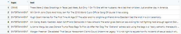
Let’s first have a look at the data. As you can see, we have 200,000 news articles and the author of the data has assigned them to 41 topics (or the topics came from the sub-section header of the news website, possibly).

Now, in a real-world scenario, you would usually not already have these labels – that’s the whole point of making the algorithm. So at this stage, we would need to select a sample of the total dataset for manual annotation:

#Select sub-set for training and testing
set.seed(2021)
sample <- sample(1:nrow(d), 10000, replace = F)

d_labelled <- d[sample,]
d_labelled$id <- sample

#Change the data structure so that you have one column for each topic
d_labelled %<>% pivot_wider(values_from = topic, names_from = "topic", 
                            names_prefix = "topic_", values_fn = length, values_fill = 0)

#If the data were not pre-annotated, you would need to manually go through this dataset and assign the topics!
#Then you would load the dataset with your annotations again into the R session here.  

This creates a sample of 10,000 out of the total 200,000 texts. Also, we transform the data to a “wider” form so that for each topic, we have one column, as in the example with the songtexts above. So now the data look like this:

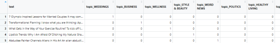
Again, in a real-world scenario you would not already have the 0’s and 1’s in the “topic_” columns. Which means that at this point, you would need to do the manual annotation of the data! For instance, you could save the data to a spreadsheet using write.csv() or writexl::write_xlsx(), open it with Excel or something similar, create the “topic_” columns (since they wouldn’t be there already), go through all the 10,000 texts (or probably fewer in a real-world case), and fill in the 1’s into the table (the 0’s can later be batch-filled with, e.g., my_data[which(is.na(my_data))] <- 0). So this is usually clearly the biggest part of the whole project (which we are skipping here so that you have a reproducible example without the need to manually create labels). With your real data, when you’re done annotating, load the annotated data back into R and it should look like the screenshot above.

So now we have created an annotated dataset for training and testing of the algorithm. This dataset is now divided into 70% training data and a 30% hold-out dataset for evaluation purposes.

#Now further divide the dataset with the topic labels into training and testing.
set.seed(2021)
sample2 <- sample(1:nrow(d_labelled), round(0.7*nrow(d_labelled),0), F)

d_train <- d_labelled[sample2,]
d_test <- d_labelled[-sample2,]

Pre-process the raw text data

In order to train an algorithm on textual data, we first need to convert the plain text into a machine-readable form. The most simple way to do that is the so-called bag-of-words representation of text. We are going to create this simple model now, because it often already yields satisfactory results. If you want to go further and try out more sophisticated, state-of-the-art neural networks, it is still useful to have this simple model as a baseline to see how big your improvement can be with the more complex model. The simple model also has the advantages that you can a) easily interpret the results and explain it to management, and b) deploy the model with fewer resources (e.g., the model which we build below can be deployed as a shiny app with minimal memory requirements, whereas using a state-of-the-art model usually requires you to host a server with a Python installation, more and resource-intensive packages, and large pre-trained models from e.g. Google needing lots of memory).

We start by creating a dictionary of all our words in the training data. The following function achieves this by:

• Splitting all texts by white space into “tokens”, and converting all upper case to lower-case characters. For instance: “This is an exemplary sentence!!” –> [“this”, “is”, “an”, “exemplary”, “sentence!!”]
• Next, we remove any characters that are not letters. Then we remove stop-words that occur so frequently that they have little information for us (e.g., “the”, “in”, etc.). So for instance: “this” “is” “an” “exemplary” “sentence!!” –> “exemplary” “sentence”
• We then stem our words, such that “sentences”, “sentence”, or “sentencing” are all reduced to “sentenc”.
• Finally, we make a count of all words across all texts and keep only those that occur at least 20 times in our dataset (change this value if you have a lot more or fewer texts).

create_dictionary <- function(data){
  corpus <- data$text
  
  #Tokenization
  corpus <- purrr::map(corpus, function(x) str_split(tolower(x),"\\s+") %>% unlist) 
  
  #Remove anything except letters
  corpus <- purrr::map(corpus, function(x) gsub("[^a-z]","",x))
  
  #Remove stop-words ("the", "in", etc.)
  corpus <- purrr::map(corpus, function(x) x[!(x %in% stopwords::stopwords("en"))])
  
  #stem
  corpus <- purrr::map(corpus, function(x) text_tokens(x, stemmer="en") %>% unlist)
  
  #Count word frequency and remove rare words
  words <- as.data.frame(sort(table(unlist(corpus)), decreasing=T), stringsAsFactors = F)
  words <- words$Var1[which(words$Freq >=20)]
  
  return(words)  
}

Try out the new function on our training data:

dict_train <- create_dictionary(d_train)
dict_train[1:10]

So “can”, “new”, and “Trump” are the most frequent words in our training data which are not stop-words. (You can of course add additional words to the list of stop-words in the function above if you wish to have them removed as well).

Creating a document-term-matrix

The next step is to use this dictionary and create a matrix that tells you whether the respective words occur in a given text, and if so, how often.

create_dtm <- function(data, dict){
  corpus <- data$text
  
  #Repeat pre-processing from above
  corpus <- purrr::map(corpus, function(x) str_split(tolower(x),"\\s+") %>% unlist) 
  corpus <- purrr::map(corpus, function(x) gsub("[^a-z]","",x))
  corpus <- purrr::map(corpus, function(x) x[!(x %in% stopwords::stopwords("en"))])
  corpus <- purrr::map(corpus, function(x) text_tokens(x, stemmer="en") %>% unlist)
  
  #Keep only words from the dictionary
  corpus <- purrr::map(corpus, function(x) x[x %in% dict])
  
  #Make dtm
  dtm <- as.data.frame(matrix(0L, nrow=nrow(data), ncol=length(dict)))
  names(dtm) <- dict
  
  freq <- purrr::map(corpus, table)
  for (i in 1:nrow(dtm)){
    dtm[i, names(freq[[i]])] <- unname(freq[[i]])
  }
  
  return(dtm)
}

What this function does is best explained when looking at the result. Apply it to our training data and our newly created dictionary:

dtm_train <- create_dtm(d_train, dict_train)
dtm_train[1:5,1:10]

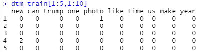
Here you can see how a document-term-matrix looks like. We have limited it to the first 5 rows (= texts) and 10 columns (most frequent words). So the first line tells us that the word “photo” occured once in the first news article. In the fourth article in our training data, there is the word “new” twice, and so on.

And that’s it already, we have the “bag-of-words” representation of our texts. Note that we disregard any n-grams (i.e. frequent sequences of words such as “I don’t like”), part-of-speech tagging (is “sentence” a noun or a verb in the given sentence?), synonyms, sarcasm, and many more things that we might want to consider when forming a more complex NLP model (a few links are given below).

Another important thing to note: We have not considered any meta data here. These could include, for instance: Name of the news media outlet, length of the article, and so on. These could systematically be related to the topic of an article. You could join this type of information to your dtm object with a simple cbind().

But let’s leave it at that and train our first algorithm!

Training an algorithm to detect one topic at a time

Tree-based models such as a random forest or a gradient boosted machine are good candidates to start with, because they are fast and easy-to-understand algorithms that usually still deliver good results. Using an extreme gradient-boosted tree (xgbTree) will make model training yet a bit faster as compared with a random forest, so let’s start with this one. I’ll explain briefly what is being done once you see the results. Let’s wrap the training into a function which also lets you decide which of the 41 topics you want to predict. Note that we start here with a binary classification, i.e. an algorithm that only detects whether or not a text belongs to one single topic “X”. Later, we will extend it to detect all topics simultaneously.

train_model <- function(data, dtm, target_topic){
 t <- factor(unlist(data[,target_topic]), levels=c(1,0))
 
 caret::train(dtm, t, method="xgbTree",
                     trControl = trainControl(method="cv", number=5, 
                                              search = "random", 
                                              verboseIter=T))
}

This simple function trains a boosted tree algorithm without tuning hyperparameters, i.e. without a procedure to determine which are the best values to choose for the various options that can be set (e.g., “max_depth” which controls how big the decision trees are to be grown, etc.). Rather, the standard procedure of trying a few random values for the parameters and then selecting the set that results in the best in-sample accuracy is used. Below I will also give you a code example for how to set these values manually.

It should be noted that I’m using the caret package here; but as you might know, the author of that package, Max Kuhn, has moved on to developing and maintaining the tidymodels package. I haven’t really gotten around to trying out the latter. Since we’re not doing something overly sophisticated here but rather only use the wrapper function train(), you should easily be able to reproduce the steps here with your preferred machine-learning package.

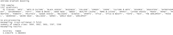
Let’s try it out! Our new function needs the training data, the document-term-matrix we created above, and your input regarding what topic you want to detect. Let’s start by classifying whether or not a news article is about politics:

set.seed(2021)
mod <- train_model(d_train, dtm_train, "topic_POLITICS")
mod

All right, so apparently we were able to detect the “politics” category with an accuracy of 89% in the training data (with the best of the three specifications tried out – note here that there is quite some variation between these three runs in terms of accuracy, so it appears as if you might get a few additional percentage points by setting up a tune grid for hyperparameter tuning, and trying if yet higher values for nrounds, lower values for gamma, etc. could give you additional accuracy).

So is 89% accuracy good? You might be tempted to say “well, this is not bad”, but remember to check for class distribution: the “politics” topic occurs in only 17% of all posts in the database. So that means that if we were always guessing “this post is not about politics”, we would be correct in 83% of all cases. With our machine-learning algorithm, we are correct in 89% of all cases. Put like this, the 89% certainly sound less impressive…

At this point, we could try out other algorithms (in addition to hyperparameter tuning) and see whether you might arrive at better results. But let’s jump straight to the model evaluation with our hold-out test data. I’ll explain later what exactly the algorithm has done so far.

As you probably know, an algorithm’s performance in machine learning is always evaluated against a test dataset that was not used to train the model. Remember that above, we have put 3,000 texts aside and reserved them for testing purposes. We are now writing a small function to transform the test data to a dtm as well, using the dictionary from the training data (this is important! Don’t create a dictionary from the test data, you need to use all information from the training data only), predicting the topics of the news articles in the test data with our algorithm – and finally comparing our predictions to reality (i.e. the topics that were assigned to the texts by the creator of the dataset).

evaluate_model <- function(model, data_test, dict, target_topic){
  t <- factor(unlist(data_test[,target_topic]), levels=c(1,0))
  dtm_test <- create_dtm(data_test, dict)
  
  predictions <- predict(mod, newdata = dtm_test)
  confusionMatrix(predictions, t)
  
}

Let’s try it out for the “politics” topic:

evaluate_model(mod, d_test, dict_train, "topic_POLITICS")

This is the result:

Here you see a confusion matrix, which is widely used to evaluate the usefulness of a machine-learning algorithm. The values in this matrix tell us that there were 266 articles in the test data where our algorithm said “this text is about the politics” and it was correct (according to the person who created the dataset). There were, however, 87 cases were the algorithm falsely claimed to have identified a text about politics (“false positives”). And, more importantly, there were 233 posts that were actually about politics but our algorithm didn’t think so (“false negatives”). So, again, although the overall accuracy of 89% might look good, the performance is actually only mediocre since 83% can be achieved by purely guessing. Here you can see why it is important to reserve a part of your annotated dataset for model evaluation, because you need the “ground truth” to compare your algorithm’s predictions against.

You’re probably familiar with the terms “sensitivity” or “specificity” through the whole Covid-19 situation. These are also given in the output. Here you can see that specificity is ok (96.5%), but sensitivity is low. This is the equivalent of an antigen test recognizing only 53% of true infections with SARS-COV-2. You wouldn’t want to rely on that test. In other words, the precision of our algorithm is low (if you are more familiar with the metrics precision, recall, or F1, you can also get these with the commandos precision(predictions,t), recall(predictions,t) or F_meas(predictions,t) inside the evaluate_model()-function above. Just make sure to pass them to the return() statement).

What can I do if my results are bad?

What can you do about the so-far not ery satisfactory results? There are always two things that you can try:

a) Use a better algorithm – so far we have used a simple one which disregards a lot of important information in the text, e.g. the similarity of words or the context in which they appear. And we have not done any hyperparameter tuning at all.
b) Assemble more training data.

Often, “more training data” beats “better algorithm”. In our example here, we could easily increase the size of the training dataset because we have 200,000 labelled texts. But, of course, in a real-world setting, if you need to generate additional training data yourself, this is time-consuming and/or costly.

So if more training data is not an option, you can try tweaking your model by hyperparameter tuning (see also below), or in the end you might need to get familiar with more complex models. Head over to RStudio’s AI blog to get started with text classification using neural networks. For the current state-of-the-art models, the so-called transformer neural networks like BERT and GPT-2, see this excellent blog post on theanalyticslab.nl by Jurriaan Nagelkerke and Wouter van Gils. It’s one of the few ressources on transformer models with R, so the authors are to be applauded for making this available to the R community.

Understanding and presenting your results

Before we move on to predicting new data and expanding the algorithm to detect all topics, let’s try to get a better grasp of what the algorithm actually does. Imagine you have to explain your results to management, but you don’t really understand what’s going on.

A great way to understand a tree-based classifier (such as a random forest or a gradient boosted tree) is to grow and plot an exemplary tree. A decision tree is an algorithm that partitions data into dissimilar sub-parts using one of the features in the dataset and repeats this process until either all resulting datasets are homogenous (e.g., all texts in end node 1 are about politics, all in end node 2 are about business, and so on) or some criterion to stop has been reached. Have a look at this example:

library(rpart)
library(rpart.plot)

set.seed(2021)
tree_data <- cbind(t = factor(unlist(d_train[,"topic_POLITICS"]), levels=c(1,0)), dtm_train)
tree <- rpart(t~., tree_data)
rpart.plot(tree)

This gives us the following tree:

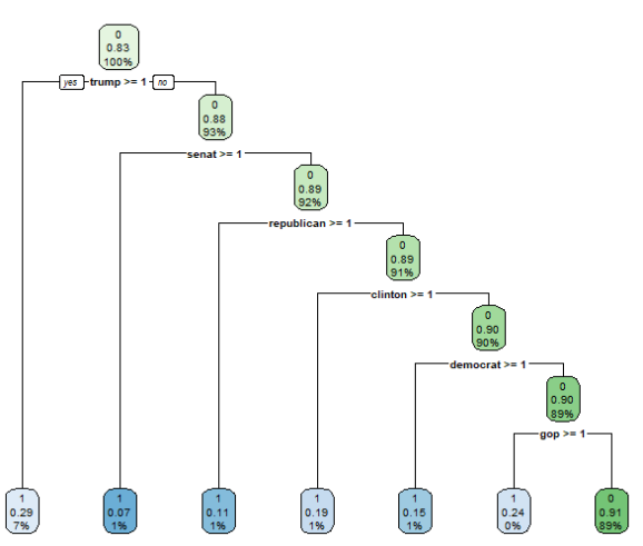
How do you read this tree? Starting from the top, the feature that best divides our data into two dissimilar parts is the word “trump”. If this word is present in a news article, move on to the branch to the left. If it’s not present, continue with the branch to the right. If Donald Trump is mentioned in an article, the probability is 71% that this article is about politics (The percentage of 0.29 given in the end note here refers to the share of “not-politics” articles since this is the second factor level. So the three numbers here tell us: We will predict a “1” (meaning yes, the article is about politics), 29% of articles in this node are not about politics, and the node comprises 7% of all articles in our trainind data). If the word “Trump” is not present, the algorithm moves on to check for the word stem “senat”, and so on.

Now obviously this is an overly simple decision tree. But for demonstration purposes, when you run this with your own data, I think it is a good way of understanding and also explaining to others, what the algorithm does. Of course, when you present this to others (e.g. management), make sure to say that your entire algorithm does not consist of only this single tree. Rather, you usually have a collection (an ensemble) of many trees. A random forest, for instance, grows many (e.g., 500) trees where each tree uses only a (randomly sampled) fraction of all features (here: words from our dictionary). So in our example, there would be many trees that are fit to the data without considering the words “Trump” or “Clinton”, so there are also decision-rules for when a text does not contain these words. This makes the algorithm more versatile and able to generalize to new texts. It reduces the focus on idiosyncrasies of the training data (for instance, in our case, due to the time frame when the data have been collected, the terms “Trump” and “Clinton” might be very dominant, masking the effect of other terms that are more time-independent and are more likely to be indicative of a politics-related news article in a different time or country). When presented with a new text, all trees take a “vote” on how to classify this text, and this is transformed into a prediction probability (e.g. “we’re 97% sure this text is not about politics).

A gradient-boosted tree is similar to a random forest, but proceeds sequentially. It first grows a tree and then puts more weight on the samples (texts in the training data) which are badly predicted by the tree before growing the next tree. By doing so, we increase the algorithm’s power to also recognize unusual examples. Keep in mind that there is always a trade-off between the accuracy of the algorithm in the training data, and the capability of generalizing to new, unseen data (see also “bias-variance tradeoff”). You can of course define a huge (i.e. fully grown) decision tree which correctly classifies all your texts in the training data (= 100% accuracy). But this will of course result in over-fitting. For example, the first text about politics in our data contains the sentence “the government was unable to locate nearly 1,500 children who had been released from its custody” – overfitting an algorithm to this text would mean it might come up with a rule such as “whenever the number 1,500 and the words ‘released’ and ‘custody’ appear in a sentence, mark as ‘politics” – and it would certainly be a bad idea to generalize this rule to all new texts in the future. In our code above, we have made sure that over-fitting is likely not a big issue by using cross-validation in the model training (“method = ‘cv'”).

Show me examples of wrong classifications

If you want to get more insights into why your algorithm wrongly classified some cases, a simple way of doing that is to read a few mis-classifications in the test data. This might give you hints about what types of texts are not understood correctly by the machine. You might act on that by assembling more training data specifically for these types of texts (which is called over-sampling; but keep in mind that you do not have a random sample anymore if you do that, which can be associated with other problems).

Let’s try this: First, we look at some texts where our algorithm falsely believed these were news paper articles about politics:

dtm_test <- create_dtm(d_test, dict_train)
predictions <- predict(mod, newdata = dtm_test)

d_test[which(d_test$topic_POLITICS == 0 & predictions == 1),][1:5,] %>% View

Which gives us:

So here of course you see an issue that always occurs with human-annotated data. The first text is about voting. The second one about Donald Trump firing someone from his staff and mentioning him being the GOP presidential candidate. Yet these articles do not fall into the “politics” category according to the author of the dataset (who generously provided this for us, let’s not forget to thank them for that). The second text here, for instance, is labelled as “entertainment”. You might have a different opinion about that and you might think that these examples are actually not “false positives”, but rather “true positives” but “questionable annotations”. As noted above, you will always run into this type of problem with supervised text classification. So no algorithm will be able to achieve a 100% accuracy if you and the coder already disagree on some of the topic annotations. So at this point there is nothing you can do in terms of modeling; rather, you might need to re-evaluate the annotations in the training data which would of course be a lengthy and costly procedure.

Swap the “0” and “1” in the code snippet above and you get examples of “false negatives”. Of course you can leave out the [1:5,] filter which would give you all false negatives instead of only the first five.

Apply the algorithm to new texts

The whole idea of training a model like this is usually to be able to label new data, i.e. feed new texts to the algorithm and it gives you the topics they are about. You could then put the model to productive use (e.g., in a shiny app).

Here, I have copied two random news texts and put them into a data frame. The way we coded our modeling functions, we need to have the texts in a data.frame in a column called “text”:

my_new_data <- data.frame(text=c("Scientists: Vaccine inequity and hesitancy to blame for variant. The emergence of Omicron highlights the failure of rich nations to share doses with the developing world",
                    "Moderate House Republican warns McCarthy over embracing far-right members. House Minority Leader Kevin McCarthy speaks on the House floor during debate on the Democrats' expansive social and environment bill at the US Capitol on November 18, 2021."))

What does our model say; are these two texts about politics or not?

predict(mod, newdata = create_dtm(my_new_data,dict = dict_train))

So the model says the first article is not about politics, whereas the second one is, which makes sense.

A model for ALL topics

So far we have limited our model to one topic. But you probably want a function which you can feed a new article to and it doesn’t just tell you “this is probably not about politics”; but it rather tells you “this is about sports”, or “this is about religion”, etc.

Before we do that, note an important characteristic from our dataset: Each text is assigned to exactly one, and only one, topic. There are no articles that are about “Sports” and “Entertainment”, etc. Which is why in the following code, we can undo the “widening” of the data which we did in the beginning, and use the vector of labels (“STYLE & BEAUTY”, “IMPACT”, “BUSINESS”, …) as the target for training the model:

t = d$topic[sample][sample2]
set.seed(2021)
mod_all <- caret::train(dtm_train, t, method="xgbTree", 
                    tuneGrid = expand.grid(eta = 0.3, max_depth = 6,gamma = 2, colsample_bytree = 0.65, 
                                           min_child_weight = 2, subsample = .95, nrounds = 700),
                    trControl = trainControl(method="cv", number=5,verboseIter=T))
mod_all

What did we do here? First we took the vector of topics, filtered to be our sample dataset (“sample”) and from this again filtered to only contain the training data (“sample2”), and passed it to the model training. Everything else is unchanged from the model training function above except one thing: Here, I do not use the “search = ‘random'” argument which causes the model training to try 3 different random sets of hyperparamters. Rather, I explicitly told the training function which values to use for the parameters eta, max_depth, and so on. I did it primarily for performance reasons here because on my laptop, training this model takes a while, so I wanted to use one specification only instead of three. You can also use this tuneGrid argument to give more values for the algorithm to try out, e.g., by specifying eta = c(0.01,0.1,0.3). If you do this, then in the output of this code snippet you see which of the eta’s resulted in the highest accuracy in the training data. But note that if you provide e.g. 3 values for each of the 7 hyperparameters, this will result in 3^7 = 2187 model specifications for the training procedure to try out. This means that serious hyperparameter tuning with a large(-ish) dataset requires you to have some serious (cloud) computing power.

My single guess of what might be a good set of parameters resulted in the following in-sample accuracy:

Accuracy = 43%, now you might be tempted to say “this is really bad”. But keep in mind that we have 41 topics and the most frequent occurs in 17% of all texts, so it’s at least, well, mediocre.

Now on to the confusion matrix, which is a bit more complicated with 41 topics as opposed to the binary (true/false) classification we had done above. Let’s see which topics were accurately predicted, and where we wrongly predicted a different topic, when we let the algorithm process our hold-out test dataset:

predictions <- predict(mod_all, newdata = dtm_test)
t_test <- as.factor(d$topic[sample][-sample2])

cm <- data.frame(confusionMatrix(predictions,t_test)$table)

#Standardize the values
for (i in unique(cm$Prediction)){
  cm$Freq[cm$Prediction==i] <- cm$Freq[cm$Prediction==i] / sum(cm$Freq[cm$Prediction==i],na.rm=T) *100
  cm$Freq[cm$Prediction==i & is.nan(cm$Freq)] <- 0
}

ggplot(cm,aes(x=Prediction,y=Reference,fill=Freq, label=paste(round(Freq,0),"%"))) +
  geom_tile() + geom_label() +
  labs(fill="Percentage:") +
  theme(axis.text.x = element_text(angle = 90))

We get this result:

Here we can clearly see which topics were accurately predicted, and where the algorithm had its problems. For instance, 78% of our predictions with label “divorce” were correctly identified as articles about divorce, whereas 5% “divorce” predictions were actually about weddings, 2% were actually “comedy”, and so on. You also find example were we hardly ever identified the topic correctly. For instance, only 13% of our “healthy living” predictions were correct; 44% of our predictions actually belonged into the “wellness” category. Again, you can see that many of our mis-classifications are likely due to the topics being not very distinct, and the annotations in some cases questionable. There is a topic “parents” and a topic “parenting”? There are “worldpost”, “the worldpost”, and “world news”…? No wonder our overall accuracy is only moderate. Here it would definitively make sense to collapse some categories, and to re-evaluate some annotations, but of course this is just an example here.

Finally, let’s use the model to make new predictions. Above I had copy-pasted two random news articles. This is how you let your model tell you what these texts are about:

predict_all_topics <- function(new_texts, dict){
  dtm <- create_dtm(data.frame(text=new_texts), dict=dict)
  predict(mod_all, newdata = dtm)
}

predict_all_topics(my_new_data, dict_train)

You get a vector with the same length as your input character vector containing the news articles. Here, the predictions are correct, but that wasn’t too hard.

A function that can predict multiple topics

OK I have one remaining point I want to share with you. Our example dataset was structured such that each news article was assigned to exactly one topic. But often, in real-world scenarios, you might want to be able to detect multiple topics from a single text. For instance, a customer might write an e-mail complaining about a defect product, asking about how to change a spare part, and also wanting to place another order. Let’s see if we can get our model to predict multiple topics from each newspaper article.

I don’t know if there is an easier way to do this, but this one works. We go back to the “wide” form of the data introduced in the beginning. This is important because this enables a text (row) to be marked as belonging to multiple columns (topics), instead of only one topic. Now we simply train one model for each topic, predicting whether or not the respective topic is present in our text:

topics <- paste0("topic_", unique(d$topic))
model_list <- list()
set.seed(2021)
for (i in 1:length(topics)){
  cat("Training model #", i, " - ", topics[i],"\n")
  t <- factor(unlist(d_train[,topics[i]]), levels=c(1,0))
  model_list[[i]] <- caret::train(dtm_train, t, method="xgbTree", 
                                  tuneGrid = expand.grid(eta = 0.3, max_depth = 6,gamma = 2, colsample_bytree = 0.65, 
                                                         min_child_weight = 2, subsample = .95, nrounds = 700),
                                  trControl = trainControl(method="cv", number=5,verboseIter=T))
}

Again, we gave only one specific set of hyperparameters to the training function, because even then training 41 models takes a while.

Let’s see what our model has to say about the two example texts:

predict_multiple_topics <- function(model_list, new_texts, dict){
  dtm <- create_dtm(data.frame(text=new_texts), dict=dict)
  purrr::map_dfc(model_list, function(x) predict(x, newdata=dtm))
}

my_predictions <- predict_multiple_topics(model_list, my_new_data, dict_train)
View(my_predictions)

Alright! In principle, there could be multiple 1’s in each row, but we only see one topic assigned to the second text. Note that in our example, it’s not surprising that our algorithm is rather conservative about giving out 1’s, because the training data was a very sparse matrix and had in fact no text assigned to two or more labels.

Note that at this stage you could again, as we demonstrated above, evaluate each of the individual models in this list in detail against the test data, check the confusion matrix, see how many false positives and false negatives were produced, examine the mis-classifications, and so on. It’s important for you to know, for instance, “my ‘science’ detector has a low sensitivity but high specificity, which means that there are most likely actually more science articles than what my algorithm’s output shows”. In addition to model tweaking such as hyperparameter tuning, you can also play with different cutoff thresholds for predicting “1” vs. “0” for a specific topic. For instance, you can change your predict()-function to return probabilities instead of 1/0:

p <- predict(mod, newdata = create_dtm(my_new_data,dict = dict_train), type="prob")
ifelse(p > 0.4, 1, 0)

This will lower the cutoff-value for assigning a topic from 0.5 to 0.4. You can then pass these values to the confusion matrix to see whether sensitivity/specificity are improved.

When you’re done, let’s move on to the final goal that you’ve been working towards.

Finally, what you usually want to do with thistype of algorithm, you want to take a whole bunch of new texts and run them through your topic classification model. “Here I have thousands of customer e-mails – dear algorithm, please tell me what they are all about.” For demonstration purposes I’ve taken all 200,000 texts from our dataset and let our algorithm decide what they are about (remember it’s been trained on “only” 10,000 of those). This is an example of how you can fo that and then bring the results to a graphical format that you could use in a presentation or report:

all_predictions <- predict_multiple_topics(model_list, d$text, dict_train)

summary_data <- apply(all_predictions %>% select(-text), 2, function(x)sum(as.numeric(x), na.rm=T)) 
summary_data <- data.frame(topic=names(summary_data), count=unname(summary_data)) %>%
  arrange(count) 
summary_data$topic <- factor(summary_data$topic, levels=summary_data$topic)

ggplot(summary_data, aes(x=topic, y=count, label=count)) +
  geom_col(fill="darkblue") + geom_label()+
  theme_classic() + coord_flip() +
  ggtitle("Topics in 200,000 news articles, by frequency",
          subtitle = "As detected by machine-learning algorithm")

Which gives us:

And that is it! Now you can use the code to, say, compare multiple news sources (which one features more articles about crime or sports?), compare data over time (did articles about “healthy living” become more frequent in the last couple years?), and so on. Or you can use the raw data (the all_predictions object above) to, say, filter articles about topic X and forward them to my friend’s inbox, etc.

Good luck with your text classification project. I hope this post might be of use to a few people – let me know in the comments if you have any questions.