
Black-Derman-Toy Interest Rate model using R
[This article was first published on K & L Fintech Modeling, and kindly contributed to R-bloggers]. (You can report issue about the content on this page here)
Want to share your content on R-bloggers? click here if you have a blog, or here if you don't.
This post implements Black-Derman-Toy (BDT) interest rate tree using R. This implementation is based on the previous post for BDT model. Want to share your content on R-bloggers? click here if you have a blog, or here if you don't.
R Implementation of BDT Interest Rate Tree
We implement BDT tree according to the content of the previous post. The previous post below explains BDT model and provides Excel illustration for the clear understanding.
Like previous post, we try to replicate BDT paper’s result.
Two Requirements for No-arbitrage Condition
As stated in previous post, for BDT short rate tree to be arbitrage free, this interest rate tree should fit a given initial term structure exactly. \[\begin{align} P_{…u} &= \frac{1}{2}\frac{P_{…uu}+P_{…ud}}{1+r_{…u}} \\ P_{…d} &= \frac{1}{2}\frac{P_{…du}+P_{…dd}}{1+r_{…d}} \end{align}\] Cross-sectional (at the same time) two adjacent short rates and spot rates are given the following intra volatility restrictions. (\(\Delta t = 1\)) \[\begin{align} \sigma_t^r = \frac{1}{2}\log\left(\frac{r_{…u}}{r_{…d}}\right) \end{align}\] \[\begin{align} \sigma_t^y = \frac{1}{2}\log\left(\frac{y_{u}}{r_{d}}\right) \end{align}\]
R code
Using the above two constraints, we use R optimization to solve for the 8 unknown variables problem. The objective function returns sum of two distances between market and model quantities: discount factors and yield volatilities.
1 2 3 4 5 6 7 8 9 10 11 12 13 14 15 16 17 18 19 20 21 22 23 24 25 26 27 28 29 30 31 32 33 34 35 36 37 38 39 40 41 42 43 44 45 46 47 48 49 50 51 52 53 54 55 56 57 58 59 60 61 62 63 64 65 66 67 68 69 70 71 72 73 74 75 76 77 78 79 80 81 82 83 84 85 86 87 88 89 90 91 92 93 94 95 96 97 98 99 100 101 102 103 104 105 106 107 108 109 110 111 112 113 114 115 116 117 118 119 120 121 122 123 124 125 126 127 128 129 | #========================================================# # Quantitative ALM, Financial Econometrics & Derivatives # ML/DL using R, Python, Tensorflow by Sang-Heon Lee # # https://kiandlee.blogspot.com #——————————————————–# # Black-Derman-Toy Interest Rate Tree #========================================================# graphics.off() # clear all graphs rm(list = ls()) # remove all files from your workspace #———————————————— # construct short rate tree (rt) #———————————————— generate_BDT_tree <– function(v.rd, v.rv, nmat) { df.rt <– matrix(0, nmat, nmat) df.rt[1,1] <– v.rd[1] # r0 for(t in 2:nmat) { df.rt[t,t] <– v.rd[t] for(s in (t–1):1) { # cross-sectional iteration df.rt[s,t] <– df.rt[s+1,t]*exp(2*v.rv[t]) } } return(df.rt) } #———————————————— # discount cash flow at maturity using BDT tree #———————————————— pricing_BDT_tree <– function(df.BDT_tree, v.cf, nmat) { df.rt <– df.BDT_tree t <– nmat df.pt <– matrix(0, t+1, t+1) df.pt[,t+1] <– v.cf # cash flow at maturity for(b in t:1) { # backward induction for(s in 1:b) { # cross-sectional iteration df.pt[s,b] <– 0.5* (df.pt[s,b+1]+df.pt[s+1,b+1])/(1+df.rt[s,b]) } } return(df.pt) } #———————————————— # objective function #———————————————— # v.unknown : rd, rdd, …, rv2, rv3, … # df.mkt : data.frame for mat, y, yv #———————————————— objfunc_BDT_tree <– function(v.unknown, df.mkt) { v.unknown <– v.unknown^2 # non-negativity nmat <– length(df.mkt$mat) # short rate and its volatility v.rd <– c(df.mkt$y[1], v.unknown[1:(nmat–1)]) v.rv <– c(df.mkt$yv[1],v.unknown[nmat:(2*(nmat–1))]) # construct rate tree(rt) df.rt <– generate_BDT_tree(v.rd, v.rv, nmat) #———————————————— # make a price tree for each maturity # calculate discount factor difference # calculate yield volatility difference #———————————————— v.df_diff <– v.yv_diff <– rep(0,nmat–1) for(t in 2:nmat) { df.pt <– pricing_BDT_tree(df.rt, 1, t) # difference between model and # market discount factor at time 0 v.df_diff[t–1] <– df.pt[1,1] – 1/(1+df.mkt$y[t])^t # difference between yield volatilities # from up & down discount factors (model) and # market discount factors yu <– (1/df.pt[1,2])^(1/(t–1))–1 yd <– (1/df.pt[2,2])^(1/(t–1))–1 yv <– log(yu/yd)/2 v.yv_diff[t–1] <– yv – df.mkt$yv[t] } return(sqrt(sum(v.df_diff^2) + sum(v.yv_diff^2))) } #———————————————— # Main #———————————————— # Input data : maturity, yield, yield volatility df.mkt <– data.frame( mat = c(1, 2, 3, 4, 5), y = c(0.1, 0.11, 0.12, 0.125, 0.13), yv = c(0.2, 0.19, 0.18, 0.17, 0.16) ) # initial guess for short rate and volatility # short rate : rd, rdd, rddd, rdddd # short rate volatilities : rv2, rv3, rv4, rv5 v.initial_guess <– c(0.1, 0.1, 0.1, 0.1, # rd 0.19, 0.18, 0.17, 0.16) # rv v.initial_guess <– sqrt(v.initial_guess) # calibration of BDT tree m<–optim(v.initial_guess, objfunc_BDT_tree, control = list(maxit=5000, trace=2, reltol = 1e–16), method=c(“BFGS”),df.mkt = df.mkt) # transform and split parameters v.param_trans <– m$par^2 nmat <– 5 # final calibrated parameters # short rate : r0, rd, rdd, rddd, rdddd (v.rd <– c(df.mkt$y[1], v.param_trans[1:(nmat–1)])) # short rate volatilities : rv1, rv2, rv3, rv4, rv5 (v.rv <– c(df.mkt$yv[1], v.param_trans[nmat:(2*(nmat–1))])) # final BDT short rate tree (df.rt <– generate_BDT_tree(v.rd, v.rv, nmat)) # final BDT price tree (5-year) (pricing_BDT_tree(df.rt, 1, nmat)) | cs |
The above R code is implemented from the logic of the previous post.
generate_BDT_tree() function returns a BDT short rate tree with arguments of unknown short rates and its volatilities. pricing_BDT_tree() function uses backward induction to discount cash flows at maturity using the BDT short rate tree and returns a price tree. Of course, the first element of the price tree is the price of zero coupon bond.
objfunc_BDT_tree() function is the objective function to be minimized, which returns a sum of squared errors of discount factors and yield volatilities. In the objective function, unknown variables are squared because yield volatility is always non-negative and in lognormal model, interest rate is non-negative.
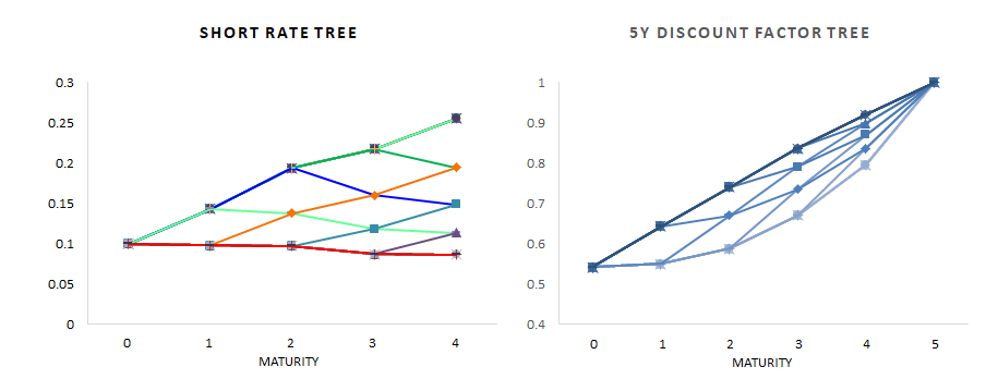
Running the above R code, we can obtain the following results which are the same as that of the previous post.
1 2 3 4 5 6 7 8 9 10 11 12 13 14 15 16 17 18 19 20 21 22 23 24 25 | > # final calibrated parameters > > # short rate : r0, rd, rdd, rddd, rdddd [1] 0.10000000 0.09791528 0.09760006 0.08717225 0.08653488 > > # short rate volatilities : rv1, rv2, rv3, rv4, rv5 [1] 0.2000000 0.1899992 0.1719859 0.1526818 0.1352092 > > # final BDT short rate tree (5-year) [,1] [,2] [,3] [,4] [,5] [1,] 0.1 0.14317978 0.19418699 0.21788708 0.25524429 [2,] 0.0 0.09791528 0.13766867 0.16055127 0.19476675 [3,] 0.0 0.00000000 0.09760006 0.11830307 0.14861875 [4,] 0.0 0.00000000 0.00000000 0.08717225 0.11340505 [5,] 0.0 0.00000000 0.00000000 0.00000000 0.08653488 > > # final BDT price tree (5-year) [,1] [,2] [,3] [,4] [,5] [,6] [1,] 0.5427603 0.5509767 0.5888395 0.6706866 0.7966577 1 [2,] 0.0000000 0.6430960 0.6708913 0.7356824 0.8369835 1 [3,] 0.0000000 0.0000000 0.7412386 0.7908217 0.8706109 1 [4,] 0.0000000 0.0000000 0.0000000 0.8363453 0.8981457 1 [5,] 0.0000000 0.0000000 0.0000000 0.0000000 0.9203570 1 [6,] 0.0000000 0.0000000 0.0000000 0.0000000 0.0000000 1 > | cs |
Concluding Remarks
From this post, we have implemented BDT short rate tree using R’s optimization routine. This will be used for pricing a fixed income derivatives such as callable bonds and for generating interest rate scenarios for multi-stage stochastic linear programming. \(\blacksquare\)
To leave a comment for the author, please follow the link and comment on their blog: K & L Fintech Modeling.
R-bloggers.com offers daily e-mail updates about R news and tutorials about learning R and many other topics. Click here if you're looking to post or find an R/data-science job.
Want to share your content on R-bloggers? click here if you have a blog, or here if you don't.