Click to see R set-up code
# Libraries
if(!require("pacman")) {
  install.packages("pacman")
}
pacman::p_load(
  data.table,
  scales,
  ggplot2,
  plotly,
  DT)

# Set knitr params
knitr::opts_chunk$set(
  comment = NA,
  fig.width = 12,
  fig.height = 8,
  out.width = '100%'
)

# Load annual data only
path <-
  "~/Desktop/David/Projects/new_constructs_targets/_targets/objects/"
red_flags <-
  readRDS(paste0(path, "nc_annual_red_flags"))
annual_data <-
  readRDS(paste0(path, "nc_annual_final"))
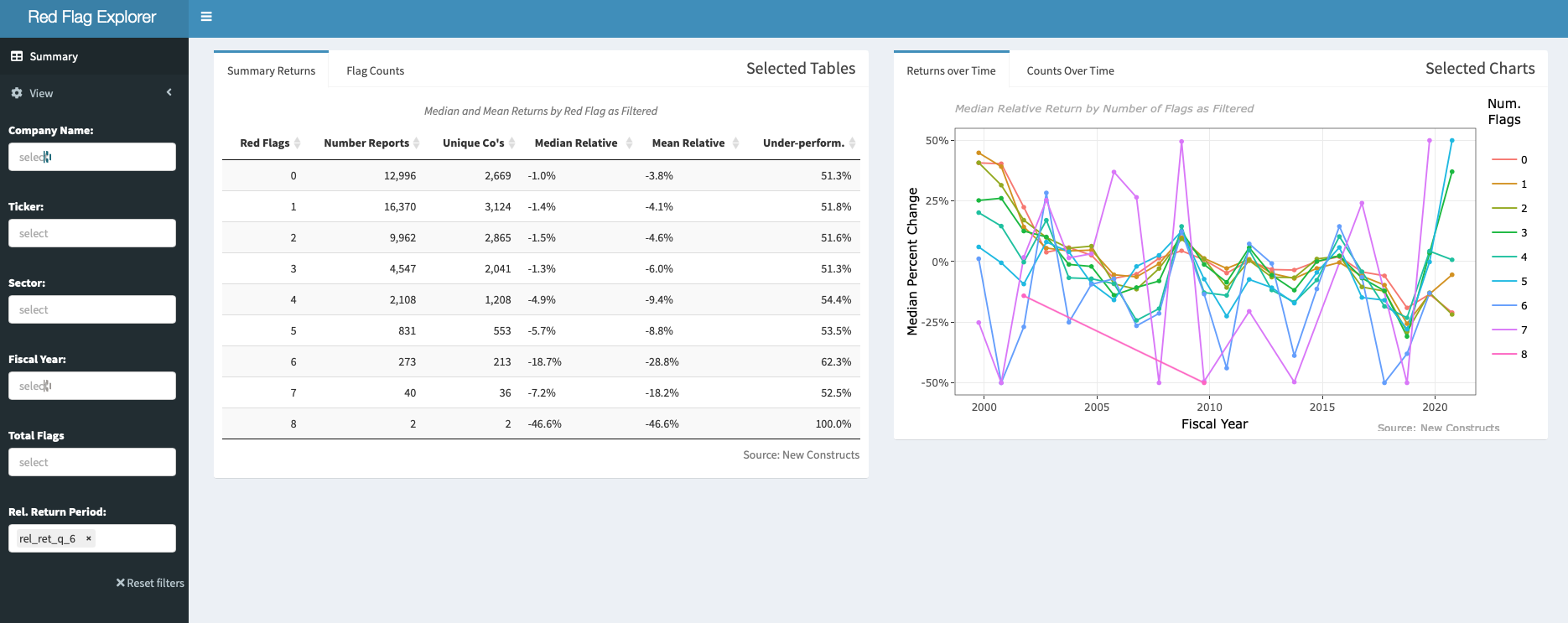
Key Findings
1999-2000 was an exceptional period for both “Red Flag” prevalence and return differentiation, though apparent benefits of the strategy appear in most periods.
Approximately 2.0% of filings we checked had 5 or more “Red Flags” among annual and quarterly filings, so sparsity is ...