Hello readers, welcome to today’s blog. I am going to implement a win probability added model for twenty 20 cricket. Now this is nothing new a quick google and there are many sources for it. Cricviz is possibly the most famous version which you may have seen on the app. The idea is the model calculates a teams chances of winning from any given position in twenty 20 match.

Each players impact on the game can then be quantified and the best players will have the highest impact on the match.

In the plot above 1 is win and 0 is loss. For 4 balls in the middle of the first innings there can clearly been seen some segmentation more runs at any stage means you have more chance of winning, there is more purple. The task then is to translate this visualisation into a usable model of how much extra chance of winning has the player added.

Data

I am using Cricsheets ball by ball data for all twenty20 matches found here:

https://cricsheet.org/

Therefore I have ball by ball data for the IPL, Internationals, the Big Bash, The Blast and the PSL. This totals over 600000 balls and should be a nice large data set to train the model.

Features

I am going to create 2 models one for the first innings and one for the second innings. For both models the main features are how many balls have been faced and how many runs they have scored as well as how many wickets they have lost. For the second innings there is the effect of scoreboard pressure and therefore I will be adding the feature of how many runs are required. Maybe its even irrelevant how many runs are required from the first ball and its all about how many runs are required at a particular stage.

Creating the models

I am using the Tidy Models collection of packages to create the initial model and subsequent models in this series. Splitting the data into training and testing sets is easy. R Sample has a function called initial split which is perfect for this example.

With initial split you specify the data that is being used for the model. The proportion with which to split the data and I have used the strata argument. This means both my training and testing data sets have a balanced amount of rows that were winning and losing. This split object can then be used with the training and testing functions to simply create the two different datasets.

I am going to train a logistic regression model to initially start. In the future I will be looking at other models and comparing them to this one.

Now that I have training and testing data I can move to the parsnip package.

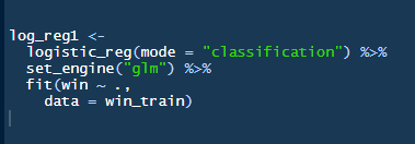
Above you can see the code to set up the first logistic regression model. The first argument logistic_reg sets up what model I was going to create. The argument mode is more used if you have a model type that can be used for both classification or regression however logistic regression is only for classification problems so the argument isn’t really needed. The next part the set_engine function and this is the great benefit of tidy models. There are many different engines with machine learning and the set engine function allows access to many of them through a common methodology. In this version I have just used a simple glm engine though there are others possible (stan, spark and keras).

Finally the fit function is just the same function you would use whatever the model. Simply it has the formula used and the data.

Results

Testing the model on the testing data by plotting a ROC curve

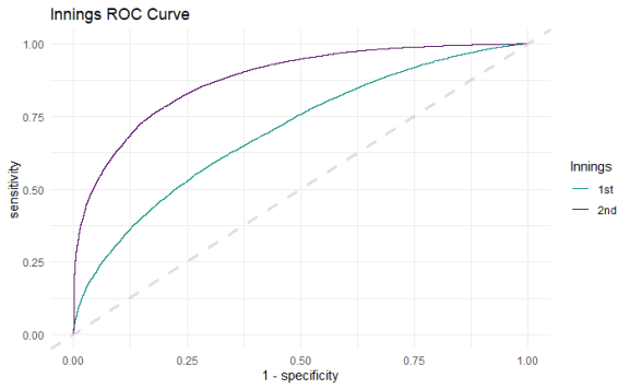
Comparing both the first and second innings model, the second innings model is clearly the better model for classifying which point is a winning score. However, this isn’t really about that the key here is both models are better then just randomly guessing and I can use this baseline to further enhance the models.

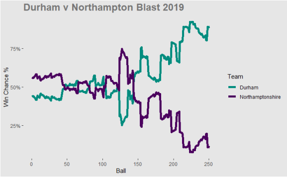
Applying the models to a match from 2019 and you can see how the win probability varies across both teams. In the first half of the innings when Durham batted it was pretty even. However, when Northampton chased Durham took control and won the match.

Above you can see a summary of each batsman’s contribution to the match. Despite what appears to be a poor batting performance Northamptonshire have 2 batsman with the best contribution. Durham batsman didnt have any big negative or positive contribution they just kept the team in the game and it looks like the bowling won the game.

Moving onto the bowlers and you can clearly see where the match winning contribution came from. Potts in 3.3 overs took 3 wickets for just 8 runs. This looks to have been the match winning contribution but looking at the information Short got man of the match.

Thats it for the first part in this series. Next part I will take this simple implementation and further review with more complicated machine learning learning models. If you have any feedback or comments please let me know. Stay Safe.