When evaluating a machine learning model if the same data is used to train and test the model this results in overfitting. So the model performs much better in predictive ability  than it would if it was applied on completely new data, this is because the model uses random noise within the data to learn from and make predictions. However, new data will have different noise and so it is hard for the overfitted model to predict accurately just from noise on data it has not seen.

Keeping the training and test datasets completely seperate in machine learning from feature selection to fitting a model mitigates this problem, this is the basis for cross validation which iteratively splits the data into different chunks and iterates over them to avoid the problem. Normally, we use 100 times repeated 10 fold cross validation for medium to large datasets and leave-one-out cross validation (LOOCV) for small datasets.

There is another technique used to correct for the “optimism” resulting from fitting a model to the same data used to test it on, this is called optimism corrected bootstrapping. However, it is based on fundamentally unsound statistical principles that can introduce major bias into the results under certain conditions.

This is the optimism corrected bootstrapping method:

1. Fit a model M to entire data S and estimate predictive ability C.
2. Iterate from b=1…B:
   1. Take a bootstrap sample from the original data, S*
   2. Fit the bootstrap model M* to S* and get predictive ability, C_boot
   3. Use the bootstrap model M* to get predictive ability on S, C_orig
3. Optimism O is calculated as mean(C_boot – C_orig)
4. Calculate optimism corrected performance as C-O.

As I have stated previously, because the same data is used for training and testing in step 3 of the bootstrapping loop, there is an information leak here. Because the data used to make M* includes many of the same data that is used to test it, when applied on S. This can lead to C_orig being too high. Thus, the optimism (O) is expected to be too low, leading to the corrected performance from step 4 being too high. This can be a major problem.

The strength of this bias for this method strongly depends on: 1) the number of variables used, 2) the number of samples used, and, 3) the machine learning model used.

I can show the bias using glmnet and random forest in these new experiments. This code is different than in Part 5 because I am changing the ROC calculation to use my own evaluation package (https://cran.r-project.org/web/packages/MLeval/index.html), and also examining random forest instead of just logistic regression.

I am going to use a low N high p simulation, because that is what I am used to working with. N is the number of observations and p the number of features. Such dimensionalities are very common in the health care and bioinformatics industry and academia, using this method can lead to highly erroneous results, some of which end up in publications.

I am simulating null datasets here with random features sampled from a Gaussian distribution, so we should not expect any predictive ability thus the area under the ROC curve should be about 0.5 (chance expectation).

Experiment 1: my implementation.

N=100 and p=5 to 500 by 50. Random forest can be selected by using ‘ranger’ or lasso by using ‘glmnet’.

## my implementation optimism corrected bootstrapping

library(ggplot2)
library(MLeval)
library(ranger)
library(glmnet)

N <- 100
alg <- 'ranger'

## loop over increasing number features
cc <- c()
for (zz in seq(5,500,50)){

print(zz)

## set up test data
test <- matrix(rnorm(N*zz, mean = 0, sd = 1),
nrow = N, ncol = zz, byrow = TRUE)
labelsa <- as.factor(sample(c(rep('A',N/2),rep('B',N/2))))
colnames(test) <- paste('Y',seq(1,zz),sep='')
row.names(test) <- paste('Z',seq(1,N),sep='')
test <- data.frame(test)
test[,zz+1] <- labelsa
colnames(test)[zz+1] <- 'XXX'
print(dim(test))

## 1. fit model to entire data and predict labels on same data
if (alg == 'glmnet'){
#orig <- glm(XXX~.,data=test,family='binomial')
X <- test[,1:zz]
Y <- labelsa
orig <- glmnet(as.matrix(X),Y,family='binomial')
preds <- predict(orig,newx=as.matrix(test[,-(zz+1)]),type='response',s=0.01)
}else{
orig <- ranger(XXX~.,data=test,probability=TRUE)
preds <- predict(orig,data=test[,-(zz+1)],type='response')
}

## 2. use MLeval to get auc
if (alg == 'ranger'){
preds <- data.frame(preds$predictions)
}else{
preds <- data.frame(B=preds[,1],A=1-preds[,1])
}
preds$obs <- labelsa
x <- evalm(preds,silent=TRUE,showplots=FALSE)
x <- x$stdres
auc <- x$Group1[13,1]
original_auc <- auc
print(paste('original:',auc))

## 3. bootstrapping to estimate optimism
B <- 50
results <- matrix(ncol=2,nrow=B)

for (b in seq(1,B)){

# get the bootstrapped data
boot <- test[sample(row.names(test),N,replace=TRUE),]
labelsb <- boot[,ncol(boot)]

# use the bootstrapped model to predict bootstrapped data labels
if (alg == 'ranger'){
bootf <- ranger(XXX~.,data=boot,probability=TRUE)
preds <- predict(bootf,data=boot[,-(zz+1)],type='response')
}else{
#bootf <- glm(XXX~.,data=boot,family='binomial')
X <- boot[,1:zz]
Y <- labelsb
bootf <- glmnet(as.matrix(X),Y,family='binomial')
preds <- predict(bootf,newx=as.matrix(boot[,-(zz+1)]),type='response',s=0.01)
}

# get auc of boot on boot
if (alg == 'ranger'){
preds <- data.frame(preds$predictions)
}else{
preds <- data.frame(B=preds[,1],A=1-preds[,1])
}
preds$obs <- labelsb
x <- evalm(preds,silent=TRUE,showplots=FALSE)
x <- x$stdres
boot_auc <- x$Group1[13,1]

# boot on test/ entire data
if (alg == 'ranger'){
## use bootstrap model to predict original labels
preds <- predict(bootf,data=test[,-(zz+1)],type='response')
}else{
preds <- predict(bootf,newx=as.matrix(test[,-(zz+1)]),type='response',s=0.01)
}

# get auc
if (alg == 'ranger'){
preds <- data.frame(preds$predictions)
}else{
preds <- data.frame(B=preds[,1],A=1-preds[,1])
}
preds$obs <- labelsa
x <- evalm(preds,silent=TRUE,showplots=FALSE)
x <- x$stdres
boot_original_auc <- x$Group1[13,1]
#

## add the data to results
results[b,1] <- boot_auc
results[b,2] <- boot_original_auc
}

## calculate the optimism
O <- mean(results[,1]-results[,2])

## calculate optimism corrected measure of prediction (AUC)
corrected <- original_auc-O

## append
cc <- c(cc,corrected)
print(cc)
}

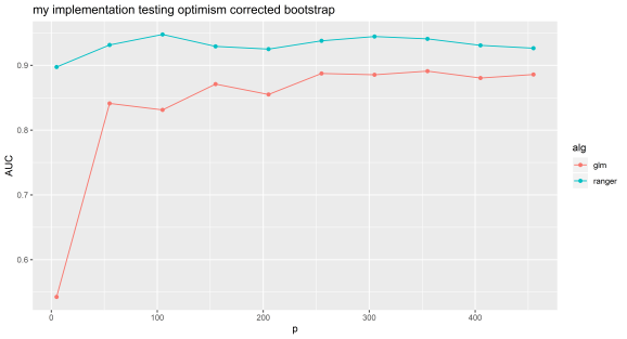
We can see that even with random features, optimism corrected bootstrapping can give very inflated performance metrics. Random data should give an AUC of about 0.5, this experiment shows the value of simulating null datasets and testing your machine learning pipeline with data with similar characteristics to that you will be using.

Below is code and results from the Caret implementation of this method (https://cran.r-project.org/web/packages/caret/index.html). Note, that the results are very similar to mine.

Caret will tune over a range of lambda for lasso by default (results below), whereas above I just selected a single value of this parameter. The bias for this method is much worse for models such as random forest and gbm, I suspect because they use decision trees which are non-linear so can more easily make accurate models out of noise if tested on the same data used to train with.

You can experiment easily with different types of cross validation and bootstrapping using null datasets with Caret. I invite you to do this, and if you change the cross validation method below, to, e.g. LOOCV or repeatedcv, you will see, these methods are not subject to this major overly optimistic results bias. They have their own issues, but I have found optimism corrected bootstrapping can give completely the wrong conclusion very easily, it seems not everyone knows of this problem before they are using it.

I recommend using Caret for machine learning. The model type and cross validation method can be changed simply without much effort. If ranger is changed to gbm in the below code we get a similar bias to using ranger.

Experiment 2: Caret implementation.

N=100 and p=5 to 500 by 50. Random forest can be selected by using ‘ranger’ or lasso by using ‘glmnet’.

## caret optimism corrected bootstrapping test

library(caret)

cc <- c()
i = 0
N <- 100

## add features iterate
for (zz in seq(5,500,50)){

i = i + 1

# simulate data
test <- matrix(rnorm(N*zz, mean = 0, sd = 1),
nrow = N, ncol = zz, byrow = TRUE)
labelsa <- as.factor(sample(c(rep('A',N/2),rep('B',N/2))))
colnames(test) <- paste('Y',seq(1,zz),sep='')
row.names(test) <- paste('Z',seq(1,N),sep='')
test <- data.frame(test)
test[,zz+1] <- labelsa
colnames(test)[zz+1] <- 'XXX'

# optimism corrected bootstrapping with caret
ctrl <- trainControl(method = 'optimism_boot',
summaryFunction=twoClassSummary,
classProbs=T,
savePredictions = T,
verboseIter = F)
fit4 <- train(as.formula( paste( 'XXX', '~', '.' ) ), data=test,
method="ranger", # preProc=c("center", "scale")
trControl=ctrl, metric = "ROC") #

cc <- c(cc, max(fit4$results$ROC))
print(max(fit4$results$ROC))
}

Further reading:

https://machinelearningmastery.com/overfitting-and-underfitting-with-machine-learning-algorithms/