
Bayesian models in R
Want to share your content on R-bloggers? click here if you have a blog, or here if you don't.

If there was something that always frustrated me was not fully understanding Bayesian inference. Sometime last year, I came across an article about a TensorFlow-supported R package for Bayesian analysis, called greta. Back then, I searched for greta tutorials and stumbled on this blog post that praised a textbook called Statistical Rethinking: A Bayesian Course with Examples in R and Stan by Richard McElreath. I had found a solution to my lingering frustration so I bought a copy straight away.
I spent the last few months reading it cover to cover and solving the proposed exercises, which are heavily based on the rethinking package. I cannot recommend it highly enough to whoever seeks a solid grip on Bayesian statistics, both in theory and application. This post ought to be my most gratifying blogging experience so far, in that I am essentially reporting my own recent learning. I am convinced this will make the storytelling all the more effective.
As a demonstration, the female cuckoo reproductive output data recently analysed by Riehl et al., 2019 [1] will be modelled using
- Poisson and zero-inflated Poisson regressions, based on the
rethinkingpackage; - A logistic regression, based on the
gretapackage.
In the process, we will conduct the MCMC sampling, visualise posterior distributions, generate predictions and ultimately assess the influence of social parasitism in female reproductive output. You should have some familiarity with standard statistical models. If you need to refresh some basics of probabilities using R have a look into my first post. All materials are available under https://github.com/monogenea/cuckooParasitism. I hope you enjoy as much as I did!
NOTE that most code chunks containing pipes are corrupted. PLEASE refer to the materials from the repo.
Introduction
Frequentist perspective
It is human nature to try reduce complexity in learning things, to discretise quantities, and this is specially true in modern statistics. When we need to estimate any given unknown parameter 
")
")
Chances are you will say } = f(H)")
Bayesian perspective
The Bayesian perspective is more comprehensive. It produces no single value, but rather a whole probability distribution for the unknown parameter ")
 = \frac{P(data | \theta) \times P(\theta)}{\int P(data | \theta) \times P(\theta) d\theta}")
or, in plain words,

The posterior can be computed from three key ingredients:
- A likelihood distribution,
;
- A prior distribution,
;
- The ‘average likelihood’,
.
All Bayes theorem does is updating some prior belief by accounting to the observed data, and ensuring the resulting probability distribution has density of exactly one.
The following reconstruction of the theorem in three simple steps will seal the gap between frequentist and bayesian perspectives.
Step 1. All possible ways (likelihood distribution)
Some five years ago, my brother and I were playing roulette in the casino of Portimão, Portugal. Among other things, you can bet on hitting either black (B) or red (r) with supposedly equal probability. For simplification, we assume =P(r)=0.5")

Having  = \frac{8}{10}")
 = 0.8")
")
A different way of thinking is to consider the likelihoods obtained using different estimates of )")
} \right)")
} \right) = 8)")
rangeP <- seq(0, 1, length.out = 100)
plot(rangeP, dbinom(x = 8, prob = rangeP, size = 10),
type = "l", xlab = "P(Black)", ylab = "Density")

As the name indicates, the MLE in the roulette problem is the peak of the likelihood distribution. However, here we uncover an entire spectrum comprising all possible ways
Step 2. Update your belief (prior distribution)
We are not even half-way in our Bayesian excursion. The omission of a prior, which is the same as passing a uniform prior, dangerously gives likelihood free rein in inference. These priors are also called ‘flat’. On the other hand, informative priors constrain parameter estimation, more so the narrower they are. This should resonate to those familiar with Lasso and ridge regularisation. Also, note that multiplying a likelihood distribution by a constant does not change its shape, even if it changes density.
Going back to the roulette example, assume I intervened and expressed my belief to my brother that  \sim Normal(0.5, 0.1)")
lines(rangeP, dnorm(x = rangeP, mean = .5, sd = .1) / 15,
col = "red")

The prior is now shown in red. In the code above, I divided the prior by a constant solely for scaling purposes. Keep in mind that distribution density only matters for the posterior.
Computing the product between the likelihood and my prior is straightforward, and gives us the numerator from the theorem. The next bit will compute and overlay the unstandardised posterior of  \times P(\theta)")
lik <- dbinom(x = 8, prob = rangeP, size = 10)
prior <- dnorm(x = rangeP, mean = .5, sd = .1)
lines(rangeP, lik * prior, col = "green")

In short, we have successfully used the ten roulette draws (black) to updated my prior (red) into the unstardardised posterior (green). Why am I calling it ‘unstandardised’? The answer comes with the denominator from the theorem.
Step 3. Make it sum up to one (standardising the posterior)
An important property of any probability density or mass function is that it integrates to one. This is the the role of that ugly denominator  \times P(\theta) d\theta")
 \times P(\theta)")
 \propto P(data | \theta) \times P(\theta)")
That funny symbol 
unstdPost <- lik * prior
stdPost <- unstdPost / sum(unstdPost)
lines(rangeP, stdPost, col = "blue")
legend("topleft", legend = c("Lik", "Prior", "Unstd Post", "Post"),
text.col = 1:4, bty = "n")

Note how shape is preserved between the unstandardised and the actual posterior distributions. In this instance we could use the unstandardised form for various things such as simulating draws. However, when additional parameters and competing models come into play you should stick to the actual posterior.
We have finally reached the final form of the Bayes theorem,  = \frac{P(data | \theta) \times P(\theta)}{\int P(data | \theta) \times P(\theta) d\theta}")
Note that in this one example there was a single datum, the number of successes in a total of ten trials. We will see that with multiple data, the single datum likelihoods and prior probabilities are all multiplied together. Moreover, when multiple parameters enter the model, the separate priors are all multiplied together as well. This might help with digesting the following example. In any case, remember it all goes into
Now is time to step up to a more sophisticated analysis involving not one, but two parameters.
Simulation
We will quickly cover all three steps in a simple simulation. This will demonstrate inference over the two parameters 

Take a sample of 100 observations from the distribution ")


")
")
")
with the last two terms corresponding to the priors of 
-
- To make all possible combinations of 200 values of
spanning 0 and 10 with 200 values of
spanning 1 and 3. These are the candidate estimates of both
- Compute the likelihood for every one of the
combinations (grid approximation). This amounts to
with i and j indexing parameter combinations and data points, respectively, or in log-scale
, which turns out to be a lot easier in R;
- Compute the product between (or sum in log-scale)
and the corresponding prior of
and of
;
- Standardise the resulting product and recover original units if using log-scale. This standardisation, as you will note, divides the product of prior and likelihood distributions by its maximum value, unlike the total density mentioned earlier. This is a more pragmatic way of obtaining probability values later used in posterior sampling.
- To make all possible combinations of 200 values of
We have now a joint posterior distribution of
# Define real pars mu and sigma, sample 100x
trueMu <- 5
trueSig <- 2
set.seed(100)
randomSample <- rnorm(100, trueMu, trueSig)

# Grid approximation, mu %in% [0, 10] and sigma %in% [1, 3]
grid <- expand.grid(mu = seq(0, 10, length.out = 200),
sigma = seq(1, 3, length.out = 200))

# Compute likelihood
lik <- sapply(1:nrow(grid), function(x){
sum(dnorm(x = randomSample, mean = grid$mu[x],
sd = grid$sigma[x], log = T))
})

# Multiply (sum logs) likelihood and priors
prod <- lik + dnorm(grid$mu, mean = 0, sd = 5, log = T) +
dexp(grid$sigma, 1, log = T)

# Standardize the lik x prior products to sum up to 1, recover unit
prob <- exp(prod - max(prod))

# Sample from posterior dist of mu and sigma, plot
postSample <- sample(1:nrow(grid), size = 1e3, prob = prob)
plot(grid$mu[postSample], grid$sigma[postSample],
xlab = "Mu", ylab = "Sigma", pch = 16, col = rgb(0,0,0,.2))
abline(v = trueMu, h = trueSig, col = "red", lty = 2)

The figure above displays a sample of size 1,000 from the joint posterior distribution |data)")
Bayesian models & MCMC
Bayesian models are a departure from what we have seen above, in that explanatory variables are plugged in. As in traditional MLE-based models, each explanatory variable is associated with a coefficient, which for consistency we will call parameter. Because the target outcome is also characterised by a prior and a likelihood, the model then approximates the posterior by finding a compromise between all sets of priors and corresponding likelihoods This is in clear contrast to algebra techniques, such as QR decomposition from OLS. Finally, the introduction of link functions widens up the range of problems that can be modelled, e.g. binary or multi-label classification, ordinal categorical regression, Poisson regression and Binomial regression, to name a few. Such models are commonly called generalised linear models (GLMs).
One of the most attractive features of Bayesian models is that uncertainty with respect to the model parameters trickles down all the way to the target outcome level. No residuals. Even the uncertainty associated with outcome measurement error can be accounted for, if you suspect there is some.
So, why the current hype around Bayesian models? To a great extent, the major limitation to Bayes inference has historically been the posterior sampling. For most models, the analytical solution to the posterior distribution is intractable, if not impossible. The use of numerical methods, such as the grid approximation introduced above, might give a crude approximation. The inclusion of more parameters and different distribution families, though, have made the alternative Markov chain Monte Carlo (MCMC) sampling methods the choice by excellence.
However, that comes with a heavy computational burden. In high-dimensional settings, the heuristic MCMC methods chart the multivariate posterior by jumping from point to point. Those jumps are random in direction, but – and here is the catch – they make smaller jumps the larger the density in current coordinates. As a consequence, they focus on the maxima of the joint posterior distribution, adding enough resolution to reconstruct it sufficiently well. The issue is that every single jump requires updating everything, and everything interacts with everything. Hence, posterior approximation has always been the main obstacle to scaling up Bayesian methods to larger dimensions. The revival of MCMC methods in recent years is largely due to the advent of more powerful machines and efficient frameworks we will soon explore.
Metropolis-Hastings, Gibbs and Hamiltonian Monte Carlo (HMC) are some of the most popular MCMC methods. From these we will be working with HMC, widely regarded as the most robust and efficient.
greta vs. rethinking
Both greta and rethinking are popular R packages for conducting Bayesian inference that complement each other. I find it unfair to put the two against each other, and hope future releases will further enhance their compatibility. In any case, here is my impression of the pros and cons, at the time of writing:
Imputation
Missing value imputation is only available in rethinking. This is an important and simple feature, as in Bayesian models it works just like parameter sampling. It goes without saying, it helps rescuing additional information otherwise unavailable. As we will see, the cuckoo reproductive output data contains a large number of NAs.
Syntax
The syntax in both rethinking and greta is very different. Because greta relies on TensorFlow, it must be fully supported by tensors. This means that custom tensor operations require some hard-coded functions with TensorFlow operations. Moreover, greta models are built bottom-up, whereas rethinking models are built top-down. I find the top-down flow slightly more intuitive and compact.
Models available
When it comes to model types, the two packages offer different options. I noticed some models from rethinking are currently unavailable in greta and vice versa. Nick Golding, one of the maintainers of greta, was kind enough to implement an ordinal categorical regression upon my forum inquiry. Also, and relevant to what we are doing next, zero-inflated Poisson regression is not available in greta. Overall this does not mean greta has less to choose from. If you are interested in reading more, refer to the corresponding CRAN documentation.
HMC sampling
The two packages deploy HMC sampling supported by two of the most powerful libraries out there. Stan (also discussed in Richard’s book) is a statistical programming language famous for its MCMC framework. It has been around for a while and was eventually adapted to R via Rstan, which is implemented in C++. TensorFlow, on the other hand, is far more recent. Its cousin, TensorFlow Probability is a rich resource for Bayesian analysis. Both TensorFlow libraries efficiently distribute computation in your CPU and GPU, resulting in substantial speedups.
Plots methods
The two packages come with different visualisation tools. For posterior distributions, I preferred the bayesplot support for greta, whilst for simulation and counterfactual plots, I resorted to the more flexible rethinking plotting functions.
Let’s get started with R
Time to put all into practice using the rethinking and greta R packages. We will be looking into the data from a study by Riehl et al. 2019 [1] on female reproductive output in Crotophaga major, also known as the Greater Ani cuckoo.
The females of this cuckoo species display both cooperative and parasitic nesting behaviour. At the start of the season, females are more likely to engage in cooperative nesting than either solitary nesting or parasitism. While cooperative nesting involves sharing nests between two or more females, parasitism involves laying eggs in other conspecific nests, to be cared after by the hosts. However, the parasitic behaviour can be favoured under certain conditions, such as nest predation. This leads us to the three main hypotheses of why Greater Ani females undergo parasitism:
- The ‘super mother’ hypothesis, whereby females simply have too many eggs for their own nest, therefore parasitising other nests;
- The ‘specialised parasites’ hypothesis, whereby females engage in a lifelong parasitic behaviour;
- The ‘last resort’ hypothesis, whereby parasitic behaviour is elicited after own nest or egg losses, such as by nest predation.
This study found better support to the third hypothesis. The authors fitted a mixed-effects logistic regression of parasitic behaviours, using both female and group identities as nested random effects. Among the key findings, they found that:
- Parasitic females laid more eggs than solely cooperative females;
- Parasitic eggs were significantly smaller than non-parasitic eggs;
- Loss rate was higher for parasitic eggs compared to non-parasitic ones, presumably due to host rejection;
- Exclusive cooperative behaviour and a mixed strategy between cooperative and parasitic behaviours yielded similar numbers in fledged offspring.
If you find the paper overly technical or literally unaccessible, you can read more about it in the corresponding News and Views, an open-access synthesis article from Nature.
Start off by loading the relevant packages and downloading the cuckoo reproductive output dataset. It is one of three tabs in an Excel spreadsheet comprising a total of 607 records and 12 variables.
library(rethinking)
library(tidyverse)
library(magrittr)
library(readxl)

# Download data set from Riehl et al. 2019
dataURL <- "https://datadryad.org/bitstream/handle/10255/dryad.204922/Riehl%20and%20Strong_Social%20Parasitism%20Data_2007-2017_DRYAD.xlsx"
download.file(dataURL, destfile = "data.xlsx")
The variables are the following:
Year, year the record was made (2007-2017)Female_ID_coded, female unique identifier (n = 209)Group_ID_coded, group unique identifier (n = 92)Parasite, binary encoding for parasitism (1 / 0)Min_age, minimum age (3-13 years)Successful, binary encoding for reproductive success / fledging (1 / 0)Group_size, number of individuals per group (2-8)Mean_eggsize, mean egg size (24-37g)Eggs_laid, number of eggs laid (1-12)Eggs_incu, number of eggs incubated (0-9)Eggs_hatch, number of eggs hatched (0-5)Eggs_fledged, number of eggs fledged (0-5)
For modelling purposes, some of these variables will be mean-centered and scaled to unit variance. These will be subsequently identified using the Z suffix.
From the whole dataset, only 57% of the records are complete. Missing values are present in Mean_eggsize (40.6%), Eggs_laid (14.8%), Eggs_incu (10.7%), Eggs_hatch (9.2%), Eggs_fledged (5.2%), Group_size (4.1%) and Successful (1.8%). Needless to say, laid, incubated, hatched and fledged egg counts in this order, cover different reproductive stages and are all inter-dependent. Naturally, there is a carry-over of egg losses that impacts counts in successive stages.
The following models will incorporate main intercepts, varying intercepts (also known as random effects), multiple effects, interaction terms and imputation of missing values. Hopefully the definitions are sufficiently clear.
Zero-inflated Poisson regression of fledged egg counts
I found modelling the number of eggs fledged an interesting problem. As a presumable count variable, Eggs_fledged could be considered Poisson-distributed. However, if you summarise the counts you will note there is an excessively large number of zeros for a Poisson variable. This in unsurprising since a lot of eggs do not make it through, as detailed above. Fortunately, the zero-inflated Poisson regression (ZIPoisson) available from rethinking accommodates an additional probability parameter $ latex p $ from a binomial distribution, which relocates part of the zero counts out of a Poisson component.
Load the relevant tab from the spreadsheet (“Female Reproductive Output”) and discard records with missing counts in Eggs_fledged. You should have a total of 575 records. The remaining missing values will be imputed by the model. Then, re-encode Female_ID_coded, Group_ID_coded and Year. This is because grouping factors must be numbered in order to incorporate varying intercepts with rethinking. This will help us rule out systematic differences among females, groups and years from the main effects. Finally, add the standardised versions of Min_age, Group_size and Mean_eggsize to the dataset.
(allTabs <- excel_sheets("data.xlsx")) # list tabs

# Read female reproductive output
fro %
as.data.frame()

fro %% mutate(female_id = as.integer(factor(Female_ID_coded)),
year_id = as.integer(factor(Year)),
group_id = as.integer(factor(Group_ID_coded)),
Min_age_Z = scale(Min_age),
Group_size_Z = scale(Group_size),
Mean_eggsize_Z = scale(Mean_eggsize))
The log-link is a convenient way to restrict the model 
")
 = \alpha_p")
 = \alpha + \alpha_{female_i} + \alpha_{year_i} + \alpha_{group_i} +")


")
")
")
")
")
")
")
In terms of code, this is how it looks like. The HMC will be run using 5,000 iterations, 1,000 of which for warmup, with four independent chains, each with its own CPU core. Finally, the precis call shows the 95% highest-density probability interval (HPDI) of all marginal posterior distributions. You can visualise these using plot(precis(...)).
eggsFMod <- map2stan(alist(
Eggs_fledged ~ dzipois(p, lambda),
logit(p) <- ap,
log(lambda) <- a + a_fem[female_id] + a_year[year_id] + a_group[group_id] +
Parasite*bP + Min_age_Z*bA + Group_size_Z*bGS + Mean_eggsize_Z*bES +
Parasite*Min_age_Z*bPA,
Group_size_Z ~ dnorm(0, 3),
Mean_eggsize_Z ~ dnorm(0, 3),
a_fem[female_id] ~ dnorm(0, sigma1),
a_year[year_id] ~ dnorm(0, sigma2),
a_group[group_id] ~ dnorm(0, sigma3),
c(sigma1, sigma2, sigma3) ~ dcauchy(0, 1),
c(ap, a) ~ dnorm(0, 3),
c(bP, bA, bGS, bES, bPA) ~ dnorm(0, 2)),
data = fro,
iter = 5e3, warmup = 1e3, chains = 4, cores = 4)

# Check posterior dists
precis(eggsFMod, prob = .95) # use depth = 2 for varying intercepts
There are no discernible effects on the number of fledged eggs, as zero can be found inside all reported 95% HPDI intervals. The effect of parasitism (bP) is slightly negative in this log-scale, which suggests an overall modest reduction in the Poisson rate.
The following code will extract a sample of size 16,000 from the joint posterior of the model we have just created. The samples of 
Then, the code produces a counterfactual plot from Poisson rate predictions. We will use counterfactual predictions to compare parasitic and non-parasitic females with varying age and everything else fixed. It will tell, in the eyes of your model, how many fledged eggs in average some hypothetical females produce. For convenience, we now consider the ‘average’ female, with average mean egg size and average group size, parasitic or not, and with varying standardised age. The calculations from the marginal parameter posteriors are straightforward. Finally, a simple exponentiation returns the predicted Poisson rates.
In summary, from the joint posterior sample of size 16,000 we i) took the
We can now examine the distribution of the sampled probabilities and predicted Poisson rates. In the case of the latter, both the mean and the 95% HPDI over a range of standardised age need to be calculated.
# Sample posterior
post <- extract.samples(eggsFMod)
# PI of P(no clutch at all)
dens(logistic(post$ap), show.HPDI = T, xlab = "ZIP Bernoulli(p)")

# Run simulations w/ averages of all predictors, except parasite 0 / 1
lambdaNoP <- exp(post$a + 0*post$bP + 0*post$bA +
0*post$bGS + 0*post$bES + 0*0*post$bPA)
simFledgeNoPar <- rpois(n = length(lambdaNoP), lambda = lambdaNoP)

lambdaP <- exp(post$a + 1*post$bP + 0*post$bA +
0*post$bGS + 0*post$bES + 1*0*post$bPA)
simFledgePar <- rpois(n = length(lambdaP), lambda = lambdaP)
table(simFledgeNoPar)
table(simFledgePar)

# Simulate with varying age
rangeA <- seq(-3, 3, length.out = 100)
# No parasite
predictions <- sapply(rangeA, function(x){
exp(post$a + 0*post$bP + x*post$bA + 0*post$bGS +
0*post$bES + 0*x*post$bPA)
})
hdpiPois <- apply(predictions, 2, HPDI, prob = .95)
meanPois <- colMeans(predictions)
plot(rangeA, meanPois, type = "l", ylim = c(0, 3), yaxp = c(0, 3, 3),
xlab = "Min Age (standardized)", ylab = expression(lambda))
shade(hdpiPois, rangeA)
# Parasite
predictionsP <- sapply(rangeA, function(x){
exp(post$a + 1*post$bP + x*post$bA + 0*post$bGS +
0*post$bES + x*post$bPA)
})
hdpiPoisP <- apply(predictionsP, 2, HPDI, prob = .95)
meanPoisP <- colMeans(predictionsP)
lines(rangeA, meanPoisP, lty = 2, col = "red")
shade(hdpiPoisP, rangeA, col = rgb(1,0,0,.25))

The left panel shows the posterior probability distribution of
We now turn to the counterfactual plot in the right panel. If for a moment we distinguish predictions made assuming parasitic or non-parasitic behaviour as 

It seems that the age of a non-parasitic ‘average’ female does not associate with major changes in the number of fledged eggs, whereas the parasitic ‘average’ female does seem to have a modest increase the older it is. Note how uncertainty increases with more extreme ages, to both sides of the panel. In my perspective, parasitic and non-parasitic C. major females are undistinguishable with respect to fledged egg counts over most of their reproductive life.
Poisson regression of laid egg counts
The following model, also based on rethinking, aims at predicting laid egg counts instead. Unlike Eggs_fledged, Eggs_laid has a minimum value of one, with a smaller relative frequency unlike the zero-inflated situation we met before. The problem, however, is that we need to further filter the records to clear missing values left in Eggs_laid. You should be left with 514 records in total. For consistency, re-standardise the variables standardised in the previous exercise.
# Try Eggs_laid ~ dpois
froReduced %
as.data.frame()

# Re-do the variable scaling, otherwise the sampling throws an error
froReduced %% mutate(female_id = as.integer(factor(Female_ID_coded)),
year_id = as.integer(factor(Year)),
group_id = as.integer(factor(Group_ID_coded)),
Min_age_Z = scale(Min_age),
Group_size_Z = scale(Group_size),
Mean_eggsize_Z = scale(Mean_eggsize))
Except for the target outcome, the model is identical to the Poisson component in the previous ZIPoisson regression:
")
")
And the corresponding implementation, with the same previous settings for HMC sampling.
eggsLMod <- map2stan(alist(
Eggs_laid ~ dpois(lambda),
log(lambda) <- a + a_fem[female_id] + a_year[year_id] + a_group[group_id] +
Parasite*bP + Min_age_Z*bA + Group_size_Z*bGS + Mean_eggsize_Z*bES +
Parasite*Min_age_Z*bPA,
Group_size_Z ~ dnorm(0, 3),
Mean_eggsize_Z ~ dnorm(0, 3),
a_fem[female_id] ~ dnorm(0, sigma1),
a_year[year_id] ~ dnorm(0, sigma2),
a_group[group_id] ~ dnorm(0, sigma3),
c(sigma1, sigma2, sigma3) ~ dcauchy(0, 1),
a ~ dnorm(0, 3),
c(bP, bA, bGS, bES, bPA) ~ dnorm(0, 2)),
data = froReduced,
iter = 5e3, warmup = 1e3, chains = 4, cores = 4)

# Check posterior dists
precis(eggsFMod, prob = .95) # use depth = 2 for varying intercepts
Here, you will note that the 95% HPDI of the bP posterior is to the left of zero, suggesting an overall negative effect of parasitism over the amount of eggs laid. The interaction term bPA too, displays a strong negative effect.
Now apply the same recipe above: produce a sample of size 16,000 from the joint posterior; predict Poisson rates for the ‘average’ female, parasitic or not, with varying standardised age; exponentiate the calculations to retrieve the predicted 
# Sample posterior
post <- extract.samples(eggsLMod)

# Run simulations w/ averages of all predictors, except parasite 0 / 1
lambdaNoP <- exp(post$a + 0*post$bP + 0*post$bA +
0*post$bGS + 0*post$bES + 0*0*post$bPA)
simFledgeNoPar <- rpois(n = length(lambdaNoP), lambda = lambdaNoP)

lambdaP <- exp(post$a + 1*post$bP + 0*post$bA +
0*post$bGS + 0*post$bES + 1*0*post$bPA)
simFledgePar <- rpois(n = length(lambdaP), lambda = lambdaP)
table(simFledgeNoPar)
table(simFledgePar)

# Sim with varying age
# No parasite
predictions <- sapply(rangeA, function(x){
exp(post$a + 0*post$bP + x*post$bA + 0*post$bGS +
0*post$bES + 0*x*post$bPA)
})
hdpiPois <- apply(predictions, 2, HPDI, prob = .95)
meanPois <- colMeans(predictions)
plot(rangeA, meanPois, type = "l", ylim = c(0, 7), yaxp = c(0, 7, 7),
xlab = "Min Age (standardized)", ylab = expression(lambda))
shade(hdpiPois, rangeA)
# Parasite
predictionsP <- sapply(rangeA, function(x){
exp(post$a + 1*post$bP + x*post$bA + 0*post$bGS +
0*post$bES + x*post$bPA)
})
hdpiPoisP <- apply(predictionsP, 2, HPDI, prob = .95)
meanPoisP <- colMeans(predictionsP)
lines(rangeA, meanPoisP, lty = 2, col = "red")
shade(hdpiPoisP, rangeA, col = rgb(1,0,0,.25))
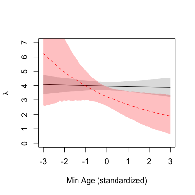
The colour scheme is the same. The mean
This time you will go one step further to simulate laid egg counts from the
# Bonus! Sample counts from predictionsP, take 95% HDPI
hdpiPoisP <- apply(predictionsP, 2, HPDI, prob = .95)
meanPoisP <- colMeans(predictionsP)
plot(rangeA, meanPoisP, type = "l", ylim = c(0, 15),
yaxp = c(0, 15, 5), xlab = "Min Age (standardized)",
ylab = expression(paste(lambda, " / no. eggs laid")))
shade(hdpiPoisP, rangeA)
poisample <- sapply(1:100, function(k){
rpois(nrow(predictionsP), predictionsP[,k])
})
hdpiSample <- apply(poisample, 2, HPDI, prob = .95)
shade(hdpiSample, rangeA)

The mean
Logistic regression of female reproductive success
We will now turn to a logistic regression of female reproductive success, using greta. Since greta limits the input to to complete cases, we need to select complete records. This gives a total of 346 records. Also, this being a different model, I used a different set of explanatory variables. The pre-processing, as you will note, is very much in line with that for the previous models.
library(tensorflow)
use_condaenv("greta")
library(greta)
library(tidyverse)
library(bayesplot)
library(readxl)

# Read female reproductive output and discard records w/ NAs
fro <- read_xlsx("data.xlsx", sheet = allTabs[2])
fro <- fro[complete.cases(fro),]

# Use cross-classified varying intercepts for year, female ID and group ID
female_id <- as.integer(factor(fro$Female_ID_coded))
year <- as.integer(factor(fro$Year))
group_id <- as.integer(factor(fro$Group_ID_coded))

# Define and standardize model vars
Age <- as_data(scale(fro$Min_age))
Eggs_laid <- as_data(scale(fro$Eggs_laid))
Mean_eggsize <- as_data(scale(fro$Mean_eggsize))
Group_size <- as_data(scale(fro$Group_size))
Parasite <- as_data(fro$Parasite)
To be consistent, I have again re-encoded Female_ID_coded, Group_ID_coded and Year as done with the rethinking models above. The logistic regression will be set up defined as follows:
")
 = \alpha + \alpha_{female_i} + \alpha_{year_i} + \alpha_{group_i} +")

")
")
And finally the model implementation. We will once again produce a posterior sample of size 16,000, separated into four chains and up to ten CPU cores with 1,000 for warmup. Note the difference in the incorporation of Female_ID_coded, Group_ID_coded and Year as varying intercepts.
# Define model effects
sigmaML <- cauchy(0, 1, truncation = c(0, Inf), dim = 3)
a_fem <- normal(0, sigmaML[1], dim = max(female_id))
a_year <- normal(0, sigmaML[2], dim = max(year))
a_group <- normal(0, sigmaML[3], dim = max(group_id))

a <- normal(0, 5)
bA <- normal(0, 3)
bEL <- normal(0, 3)
bES <- normal(0, 3)
bGS <- normal(0, 3)
bP <- normal(0, 3)
bPA <- normal(0, 3)

# Model setup
mu <- a + a_fem[female_id] + a_year[year] + a_group[group_id] +
Age*bA + Eggs_laid*bEL + Mean_eggsize*bES + Parasite*bP +
Group_size*bGS + Parasite*Age*bPA

p <- ilogit(mu)
distribution(fro$Successful) <- bernoulli(p)
cuckooModel <- model(a, bA, bEL, bES, bP, bGS, bPA)

# Plot
plot(cuckooModel)

# HMC sampling
draws <- mcmc(cuckooModel, n_samples = 4000,
warmup = 1000, chains = 4, n_cores = 10)
# Trace plots
mcmc_trace(draws)
# Parameter posterior
mcmc_intervals(draws, prob = .95)

We can visualise the marginal posteriors via bayesplot::mcmc_intervals or alternatively bayesplot::mcmc_areas. The figure above reflects a case similar to the ZIPoisson model. While parasitism displays a clear negative effect in reproductive success, note how strongly it interacts with age to improve reproductive success.
Proceeding to the usual counterfactual plot, note again that the above estimates are in the logit-scale, so we need the logistic function once again to recover the probability values.
# Simulation with average eggs laid, egg size and group size, w/ and w/o parasitism
seqX <- seq(-3, 3, length.out = 100)
probsNoPar <- sapply(seqX, function(x){
scenario <- ilogit(a + x*bA)
probs <- calculate(scenario, draws)
return(unlist(probs))
})
probsPar <- sapply(seqX, function(x){
scenario <- ilogit(a + x*bA + bP + x*bPA)
probs <- calculate(scenario, draws)
return(unlist(probs))
})

plot(seqX, apply(probsNoPar, 2, mean), type = "l", ylim = 0:1,
xlab = "Min age (standardized)", ylab = "P(Successful)",
yaxp = c(0, 1, 2))
rethinking::shade(apply(probsNoPar, 2, rethinking::HPDI, prob = .95),
seqX)
lines(seqX, apply(probsPar, 2, mean), lty = 2, col = "red")
rethinking::shade(apply(probsPar, 2, rethinking::HPDI, prob = .95),
seqX, col = rgb(1,0,0,.25))

As with the previous predicted Poisson rates, here the mean 

Wrap-up
That was it. You should now have a basic idea of Bayesian models and the inherent probabilistic inference that prevents the misuse of hypothesis testing, commonly referred to as P-hacking in many scientific areas. Altogether, the models above suggest that
- Parasitism in older C. major females has a modest, positive contribution to the number of fledged eggs. The minor negative effect of parasitism is counterbalanced by its interaction with age, which displays a small positive effect on the number of fledged eggs. Non-parasitic females, on the other hand, show no discernible change in fledged egg counts with varying age. These observations are supported by the corresponding counterfactual plot;
- In the case of laid eggs, there seems to be a strong negative effect exerted by both parasitism and its interaction with age. The counterfactual plot shows that whereas young parasitic females lay more eggs than young non-parasitic females, there is a turning point in age where parasitism leads to comparatively fewer eggs. The additional simulation of laid egg counts further supports this last observation;
- Notably, reproductive success seems to be also affected by the interaction between age and parasitism status. The results are similar to that from the ZIPoisson model, showing an increase in success probability with increasing age that outpaces that for non-parasitic females.
Thus, relatively to non-parasitic females, the older the parasitic females the fewer laid eggs, and vice versa; yet, the older the parasitic females, the more fledged eggs. Reproductive success also seems to be boosted by parasitism in older females. There are many plausible explanations for this set of observations, and causation is nowhere implied. It could well be masking effects from unknown factors. Nonetheless, I find it interesting that older parasitising females can render as many or more fledglings from smaller clutches, compared to non-parasitising females. Could older parasitic females be simply more experienced? Could they have less laid eggs due to nest destruction? How to explain the similar rate of reproductive success?
Much more could be done, and I am listing some additional considerations for a more rigorous analysis:
- We haven’t formally addressed model comparison. In most cases, models can be easily compared on the basis of information criteria, such as deviance (DIC) and widely applicable (WAIC) information criteria to assess the compromise between the model fit and the number of degrees of freedom;
- We haven’t looked into the MCMC chains. During the model sampling, you probably read some warnings regarding ‘divergence interactions during sampling’ and failure to converge. The
rethinkingpackage helps you taming the chains by reporting the Gelman-Rubin convergence statisticRhatand the number of effective parametersn_eff, whenever you invokeprecis. IfRhatis not approximately one orn_effis very small for any particular parameter, it might warrant careful reparameterisation. User-provided initial values to seed the HMC sampling can also help; - We haven’t looked at measurement error or over-dispersed outcomes. These come handy when the target outcome has a very large variance or exhibits deviations to theoretical distributions;
- We haven’t consider mixed or exclusive cooperative or parasitic behaviour, so any comparison with the original study [1] is unfounded.
Finally, a word of appreciation to Christina Riehl, for clarifying some aspects about the dataset and Nick Golding, for his restless support in the greta forum.

This is me writing up the introduction to this post in Santorini, Greece. My next project will be about analysing Twitter data, so stay tuned. Please leave a comment, a correction or a suggestion!
References
[1] Riehl, Christina and J. Strong, Meghan (2019). Social parasitism as an alternative reproductive tactic in a cooperatively breeding cuckoo. Nature, 567(7746), 96-99.
R-bloggers.com offers daily e-mail updates about R news and tutorials about learning R and many other topics. Click here if you're looking to post or find an R/data-science job.
Want to share your content on R-bloggers? click here if you have a blog, or here if you don't.