Back – Predictive Analytics Tutorial: Part 3

 

Tutorial 1:  Define the Problem and Set Up

Tutorial 2: Exploratory Data Analysis (EDA)

Tutorial 3: Transform

Tutorial 4:  Model, Assess and Implement

Welcome Back!

Great job, you’ve made it to part 4 of this 4-part tutorial series on predictive analytics!  The goal of this tutorial is to provide an in-depth example of using predictive analytic techniques that can be replicated to solve your business use case.  In my previous blog posts, I covered the first four phases of performing predictive modeling: Define, Set Up, EDA and Transformation.  In this tutorial, I will be covering the fifth and sixth phases of predictive modeling: Model, Assess and Implement.

Let’s remember where we left off –  Upon completion of the first,  second  and third tutorials, we had understood the problem, set up our Data Science Experience (DSX) environment, imported the data, explored it in detail and transformed our data to prepare for predictive modelling.  To continue, you can follow along with the steps below by copying and pasting the code into the data science experience notebook cells and hitting the “run cell” button.  Or you can download the full code from my github repository.

Log back into Data Science Experience – Find your project and open the notebook.  Click the little pencil button icon in the upper right hand side of the notebook to edit.  This will allow you to modify and execute notebook cells.

Re-Run all of your cells from the previous tutorials (except the install commands) – Minimally, every time you open up your R environment (local or DSX), you need to reload your data and reload all required packages.  For the purposes of this tutorial also please rename your data frame as you did in the last tutorial.  Remember to run your code, select the cell and hit the “run cell” button that looks like a right-facing arrow.  

 

*Tip: In DSX there is a shortcut to allow you to rerun all cells again, or all cells above or below the selected cell.  This is an awesome time saver. 

 

 

Baseline our goals – It’s important to remind ourselves of our goals from part 1.  The company is struggling with employee satisfaction.  In employee exit interviews, employees indicated they would like to get paid for their overtime hours worked.  To assess the feasibility of this, we are trying to create a predictive model to estimate the average monthly hours worked for our current employee base.  This will allow us to estimate how many overtime hours our current employee base is likely to work and how much the company would need to set aside for overtime pay.

 

Model 1: Linear Regression with all variables

During tutorial #3 we had created the data set which we will use to train our predictive algorithms.  To get started with our predictive modelling, we are just going to create a linear regression model using all the variables in the data set.  This means we are including all 32 predictive variables either from the original data set or created by us during the transformation phase.  This will likely not be the highest performing model, but it’s a great way to just get started.

model.lr1 <- lm(avgHrs ~ ., train)

Run the summary command to see how each variable is included in the model as well as some basic performance metrics.

summary(model.lr1)

Next, calculate the performance metrics.  In our case we would like to gather the following metrics:

• Adjusted R Squared - Is similar to the R Squared metric as it measures the amount of variation in the variable you are trying to predict (avg monthly hours worked), that is explained by your predictors (remaining data set).  Although it adjusts for the number of variables included as predictors. A higher adjusted r squared value is better.
• AIC - Akaike information criterion attempts to measure the bias/variance trade-off by rewarding for accuracy and penalizing for over-fitting.  I described the bias/variance trade-off was in a past blog post.  A lower AIC value is better.
• BIC - Bayesian information criterion is similar to AIC, except that it has a higher penalty for including more variables in the model. A lower BIC value is also better.
• Mean Squared Prediction Error - Displays the average squared difference between the predicted values and actual values in the testing set.  A lower  mean squared prediction error value is better.
• Standard Error - Shows the standard deviation of the prediction error above.  A lower standard error value is better.

Gather the Metrics for this model:

#Adj R-squared - higher is better.  AIC, BIC - lower the better
aic <- AIC(model.lr1)
bic <-BIC(model.lr1)

# Mean Prediction Error and Std Error - lower is better
pred.model.lr1 <- predict(model.lr1, newdata = test) # validation predictions
meanPred <- mean((test$avgHrs - pred.model.lr1)^2) # mean prediction error
stdError <- sd((test$avgHrs - pred.model.lr1)^2)/length(test$avgHrs) # std error

Note that our metrics do not tell us too much on their own.  The best practice is to run a number of models and compare the metrics to each other.  To make our lives easier, we are going to create a list to store the model metrics.  This will simplify comparing model performance when we have run all of our models. 

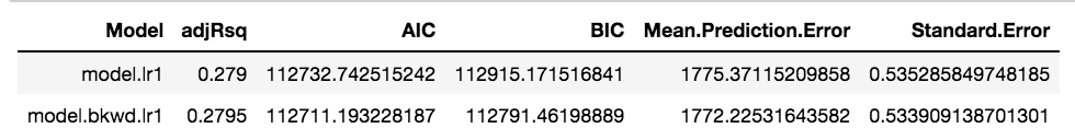
### Create a list to store the model metrics
modelMetrics <- data.frame( "Model" = character(), "adjRsq" = integer(),  "AIC"= integer(), "BIC"= integer(), "Mean Prediction Error"= integer(), "Standard Error"= integer(), stringsAsFactors=FALSE)

# Append a row with metrics for model.lr1
modelMetrics[nrow(modelMetrics) + 1, ] <- c( "model.lr1", 0.279, aic, bic, meanPred, stdError)
modelMetrics

 

Model 2: Backward Selection linear Regression

We would now like to make a linear model with a lot less variables.  It can be hard to pick which variables to include.  Rather than trying an obscene amount of variable combinations, we can use a variable selection functions to help us.  In this case we are going to use backward selection based on the AIC metric performance.  Backward selection works by starting with a larger set of predictor variables in the model and removing the least beneficial predictor one at a time during each step until it converges upon an optimal model.  We are using the method stepAIC() from the MASS package.  It requires an input of another linear model as a starting point.  This works well for us as we happen to already have a the linear model model.lr1 from the previous step which is built on all possible variables.

Start by creating the model and displaying results

step <- stepAIC(model.lr1, direction="backward")
step$anova # display results

The output displays the model performance and variables removed during each step in the backward selection method.  In the last step it shows the variables used for our final model.  We will then plug these into a new linear model.

model.bkwd.lr1 <- lm(avgHrs ~ satLevel + lastEval + numProj + timeCpny + left + satLevelLog +
lastEvalLog + satLevelSqrt + lastEvalSqrt, train)
summary(model.bkwd.lr1)

Measure the model and add the metrics to our list

#Adj R-squared - higher is better, AIC, BIC - lower the better
aic <- AIC(model.bkwd.lr1)
bic <-BIC(model.bkwd.lr1)

# mean Prediction Error and Std Error - lower is better
pred.model.bkwd.lr1 <- predict(model.bkwd.lr1, newdata = test) # validation predictions
meanPred <- mean((test$avgHrs - pred.model.bkwd.lr1 )^2) # mean prediction error
stdError <- sd((test$avgHrs - pred.model.bkwd.lr1 )^2)/length(test$avgHrs) # std error
# Append a row to our modelMetrics
modelMetrics[nrow(modelMetrics) + 1, ] <- c( "model.bkwd.lr1", 0.2795, aic, bic, meanPred, stdError)
modelMetrics

 

Model 3: Highly correlated Linear Regression

Variable selection methods are great to pare down your predictive models.  However, sometimes it can make sense to include variables based on what you learned during your exploration phases.  I tend to like trying variables which are highly correlated to the predictor and see how that performs.  Let's try that out here. 

The first step is to pull a correlation matrix on our full variable set which includes all newly created dummy, interaction and transformed variables. 

#Create correlation matrix including all numeric variables.  9-13 are not numeric.
corData <- train[ -c(9:13) ]
head(corData)
corMatrix <-cor(corData, use="complete.obs", method="pearson")
corrplot(corMatrix, type = "upper", order = "hclust", col = c("black", "white"), bg = "lightblue", tl.col = "black")

#some of the highest correlated are: 
#numProj, lastEvalLog, timeCmpy, left, greatEvalLowSat

Create the model with some of the most highly correlated variables as displayed in the above graph.

model.lr2 <- lm(avgHrs ~ numProj + lastEvalLog + timeCpny + left + greatEvalLowSat, train)
summary(model.lr2)

Measure and display the model performance.

#Measure performance. Adj R-squared - higher is better, AIC, BIC - lower the better
aic <- AIC(model.lr2)
bic <-BIC(model.lr2)
# mean Prediction Error and Std Error - lower is better
pred.model.lr2 <- predict(model.lr2, newdata = test) # validation predictions

meanPred <- mean((test$avgHrs - pred.model.lr2 )^2) # mean prediction error
stdError <- sd((test$avgHrs - pred.model.lr2 )^2)/length(test$avgHrs) # std error
# Append a row to our modelMetrics

modelMetrics[nrow(modelMetrics) + 1, ] <- c( "model.lr2", 0.2353, aic, bic, meanPred, stdError)
modelMetrics

 

 

MODEL 4: best subsets Linear Regression

We will pick back up on automated variable selection for our final model by using a best subset selection method.  Best subset identifies the best predictors to use for each n variable predictor model. It then further allows for identification of the best number of variables to include based on the desired evaluation metric. In this case we are going to look for the model with the lowest BIC metric.

Selection of best subset based on BIC values

model.bestSub=regsubsets(avgHrs ~ ., train, nvmax =25) 
summary(model.bestSub) 
reg.summary =summary(model.bestSub) 
which.min (reg.summary$bic ) 
which.max (reg.summary$adjr2 ) # just for fun

#Plot the variable bic values by number of variables
plot(reg.summary$bic ,xlab=" Number of Variables ",ylab=" BIC",type="l") 
points (6, reg.summary$bic [6], col =" red",cex =2, pch =20) 

Note that you will likely get an error message stating "Warning message in leaps.setup(x, y, wt = wt, nbest = nbest, nvmax = nvmax, force.in = force.in, ....".  This just means that there are a number of redundant variables.  In this scenario we expect this as we have all of the log, sqrt and scale transformed variables and the original variables.  We could remedy this by either reducing our nvmax or removing some of the redundant variables.  In our case it's fine because we are certainly not going to select a 25 variable model. 

From above, we can very easily see that the model with six variables has the lowest BIC value.  Next we use the coef() function to understand what variables were included in this six variable model.  

coef(model.bestSub, 6)

With this knowledge, we create the model and assess performance

bestSubModel = lm(avgHrs ~ satLevel + numProj + timeCpny + NAsupport + NAtechnical + NAhigh, data=train)
summary(bestSubModel)

#Adj R-squared - higher is better, AIC, BIC - lower the better
aic <- AIC(bestSubModel)
bic <-BIC(bestSubModel)
# mean Prediction Error and Std Error - lower is better
pred.bestSubModel <- predict(bestSubModel, newdata = test) # validation predictions
meanPred <- mean((test$avgHrs - pred.bestSubModel )^2) # mean prediction error
stdError <- sd((test$avgHrs - pred.bestSubModel )^2)/length(test$avgHrs) # std error

# Append a row to our modelMetrics
modelMetrics[nrow(modelMetrics) + 1, ] <- c( "bestSubModel", 0.1789, aic, bic, meanPred, stdError)
modelMetrics

 

Model Selection

The heavy lifting is now done, and we can select our model from the table above based on performance.  We are looking for a model with the highest adjRsq value and the lowest AIC, BIC, Mean Prediction Error and Standard Error.  From the above table the second model wins: model.bkwd.lr1!

 

selected model analysis

Before we are fully off the hook to implement this model, we need to do a bit of due dilligence to look at it's performance as a whole and against the predictor variables.

Run the standard linear regression diagnostic plots.  When you look at these plots you are hoping that you see relatively stable patterns.  These plots don't need to be exhaustively examined, we are just looking for warning signs that the model might have some deficiencies.  For example, in the "Residuals vs Fitted" plot, the variance is relatively the same regardless of the size of the fitted values.  If the residuals (error) were getting larger with the size of the fitted value, it may mean that this model is poor at predicting large values.  In the "Normal Q-Q" plot you are looking for the plotted values to follow the diagonal line.  Both the "Scale-Location" and "Residuals vs Leverage" you want the red line to be mostly horizontal with a pretty even spread.

#Create standard model plots
par(mfrow = c(2, 2))  # Split the plotting panel into a 2 x 2 grid
plot(model.bkwd.lr1)

 

Run a Cook's distance plot on the model.  These plots are great at showing you which observations/rows have a large impact on the model.  Ideally, we want all observations to be somewhat equal in their influence.  To handle the outliers seen in the plot, we could remove the rows 3502, 5994, 8981 and then run the model again.

#Create Cooks Distance Plot
cutoff <- 4/((nrow(train)-length(model.bkwd.lr1$coefficients)-2))
plot(model.bkwd.lr1, which=4, cook.levels=cutoff)

 

 

 

 

Pull a 2D visualization of your predictive model and it's relation to some key variables.  Looking at your model and key variables in 2D can really help your comprehension of the model. 

#visualize the model
visreg2d(model.bkwd.lr1, "numProj", "lastEvalLog", plot.type="persp" )
visreg2d(model.bkwd.lr1, "numProj", "lastEvalLog", plot.type="image" )

 

Show a visualization of your predictive model and it's relation to a key variables.  In this example, we can see that the number of hours worked increases as the employee has a higher number of projects.

visreg(model.bkwd.lr1, "numProj")

 

 

 

Create Predictions and Calculate total amount owed

Bring in the new data set and create the new variables

We need to do a simple data import of our current employee data set.  When we started with this tutorial, we used the data import feature in DSX.  For a refresher, see steps D-F on part 1.  To show diversity of options we are going to simply download from a URL this time around.  Note, this is just the raw employee data which does not include any extra transformations we have performed.  Therefore, after the import, we need to replicate our data transformations on this new data set.

#import in the data set
currentEmployees <- fread('https://raw.githubusercontent.com/lgellis/Predictive_Analytics_Tutorial/master/currentEmployees.csv')
currentEmployees
typeof(currentEmployees)
#convert to dataframe
currentEmployees <-as.data.frame(currentEmployees)

#Add the existing data transformations

colNames <- c("satLevel", "lastEval", "numProj", "timeCpny", "wrkAcdnt", "left", "fiveYrPrmo", "job", "salary")
setnames(currentEmployees, colNames)
attach(currentEmployees)
currentEmployees

#create factor variables with a better format

currentEmployees$leftFactor <- factor(left,levels=c(0,1),
                     labels=c("Did Not Leave Company","Left Company"))

currentEmployees$promoFactor <- factor(fiveYrPrmo,levels=c(0,1),
                     labels=c("Did Not Get Promoted","Did Get Promoted"))

currentEmployees$wrkAcdntFactor <- factor(wrkAcdnt,levels=c(0,1),
                      labels=c("No Accident","Accident"))

attach(currentEmployees)

#dummy variables
currentEmployees <- cbind (currentEmployees, dummy(job), dummy(salary))

#Log Transforms for: satLevel, lastEval
currentEmployees$satLevelLog <- log(satLevel)
currentEmployees$lastEvalLog <- log(lastEval)

#SQRT Transforms for: satLevel, lastEval
currentEmployees$satLevelSqrt <- sqrt(satLevel)
currentEmployees$lastEvalSqrt <- sqrt(lastEval)

#Scale Transforms for: satLevel, lastEval
currentEmployees$satLevelScale <- scale(satLevel)
currentEmployees$lastEvalScale <- scale(lastEval)

#Interaction Variable
currentEmployees$greatEvalLowSat <- ifelse(lastEval>0.8 & satLevel <0.2, 1, 0)

 

Create Predictions

Creating predictions with your predictive model is very simple in R.  Just call the predict() function and include the model and the data set to score as input. 

currentEmployees$Predictions <- predict(model.bkwd.lr1, currentEmployees) # test predictions

Calculate extra hours worked and amount Owed

We now have the estimated monthly hours worked for our current employee set.  Knowing that an average work month is 160 hours, we can calculate the overtime hours and an estimated payout based on known salary levels.

#Calculate Overage Hours
currentEmployees$predictedOverageHours = currentEmployees$Predictions - 160

#In case the employees worked less than 160 hours per month set negative values to 0
currentEmployees$netPredictedOverageHours <- currentEmployees$predictedOverageHours
currentEmployees$netPredictedOverageHours[currentEmployees$netPredictedOverageHours<0] <- 0

#Calculate total hours worked by each category

lowWageTotal = sum(currentEmployees[currentEmployees$salary=='low',]$predictedOverageHours) 
mediumWageTotal = sum(currentEmployees[currentEmployees$salary=='medium',]$predictedOverageHours) 
highWageTotal = sum(currentEmployees[currentEmployees$salary=='high',]$predictedOverageHours) 

#Assume low salary makes $10/hr, medium is $25/hr and high is $50/hr 
#and assume employees get time and a half during overtime

TotalPaidPerMonth = lowWageTotal*10*1.5 + mediumWageTotal*25*1.5 + highWageTotal*50*1.5
TotalPaidPerMonth
TotalPaidPerYear = TotalPaidPerMonth * 12
TotalPaidPerYear

From this output we can see that if the company were to pay their current 100 person employee base overtime, it would cost them $148,736/month and $1,784,839/year.

 

Summary

We made it!  We fulfilled our task and our work in predictive modelling is temporarily done.  Now we hand off the estimations to the business.  It is up to them to decide if they believe they want to invest in an overtime program given the expected financial cost.  Usually, there will still be some back and forth and refinement after the hand-off. This is expected and encouraged.  It means that your work is actually making an impact!

A big thank you to those who stayed with me for all four parts of this tutorial!  Please comment below if you enjoyed this blog, have questions or would like to see something different in the future.

Written by Laura Ellis