The problem of weighting the type 1,2 errors on binary classification came up in a forum I visit.

My solution:

# normal log-loss
ll <- function(y) function(p) -(y * log(p) + (1-y)*log(1-p))

plot(ll(0),0,1,col=1,main="log loss",ylab="loss",xlab="p")
plot(ll(1),0,1,col=2,add=TRUE)
legend("topleft",legend = c("y=0","y=1"), lty=1, col=1:2, bty="n")

# cost weighted log-loss
cwll <- function(y,cost) function(p) -(cost * y * log(p) + (1-cost)*(1-y)*log(1-p))

plot(cwll(0,0.1),0,1,col=1,main="cost weighted log loss\n(cost=0.1)",ylab="loss",xlab="p")
plot(cwll(1,0.1),0,1,col=2,add=TRUE)
legend("topleft",legend = c("y=0","y=1"), lty=1, col=1:2, bty="n")

Here we can see the different loss behaviours

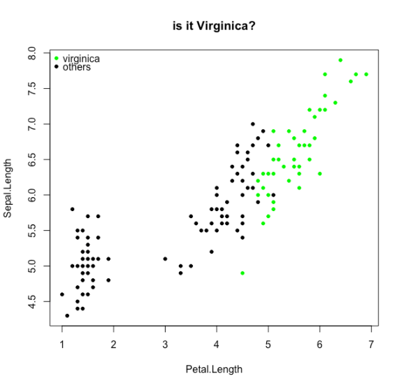
We will try to classify the Virginica species from the iris dataset

# let's take the iris data set with a species that is hard to differentiate by sepal length and petal length
d <- transform(iris, y = Species == "virginica")
plot(Sepal.Length~Petal.Length,data=d,col=0,pch=21,bg=rgb(0,y,0), main="is it Virginica?")
legend("topleft",legend=c("virginica","others"),pch=21,col=0,pt.bg=c("green","black"),bty="n")

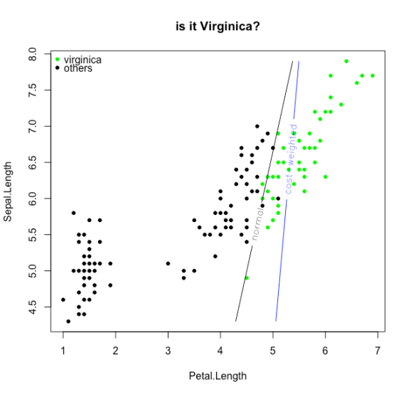
And now the loss functions:

# normal loss function
Loss <- function(par, data) {
xb <- cbind(1,d$Sepal.Length, d$Petal.Length) %*% par
p <- 1 / (1 + exp(-xb))
sum(-(d$y * log(p) + (1-d$y)*log(1-p)))
}
# cost weighted version, cost refers to error on the virginica species
cwLoss <- function(par, data, cost = 0.01) {
xb <- cbind(1,d$Sepal.Length, d$Petal.Length) %*% par
p <- 1 / (1 + exp(-xb))
sum(-(cost * d$y * log(p) + (1-cost)*(1-d$y)*log(1-p)))
}

beta <- optim(par=c(0,0,0),fn=Loss,data=d)$par
cw.beta <- optim(par=c(0,0,0),fn=cwLoss,data=d)$par

xRange <- range(d$Petal.Length)
yRange <- range(d$Sepal.Length)
X <- seq(xRange[1],xRange[2],by = 0.05)
Y <- seq(yRange[1],yRange[2],by = 0.05)
z <- outer(X,Y, FUN = function(x,y) -(beta[1] + x * beta[3] + y * beta[2]))
cwz <- outer(X,Y, FUN = function(x,y) -(cw.beta[1] + x * cw.beta[3] + y * cw.beta[2]))

contour(X,Y,z, add=TRUE,levels = 0,labels = "normal",labcex = 1)
contour(X,Y,cwz, add=TRUE,levels = 0,col=4, labels = "cost-weighted",labcex = 1)