I’m officially a Kaggler.

Cut to the good ol’ Titanic challenge. Ol’ is right – It’s been running since 2012 and ends in 3 months! I showed up late to the party. Oh well, I guess it’s full steam ahead from now on.

The competition  ‘Machine Learning from Disaster’ asks you to apply machine learning to analyse and predict  which passengers survived the Titanic tragedy. It is placed as knowledge competition.

Since I am still inching my way up the learning curve, I tried to see what I could achieve with my current tool set. For my very quick first attempt, it seemed like a no-brainer to apply out of the box logistic regression. For those in the competition, this approach, got me at around 75.something% and  placed me at 4,372 of 5172 entries. I have 3 months to better this score. And better it, I shall!

So essentially how this works is that you download the data from Kaggle. 90% of it (889 rows)  is flagged as training data and the rest is test data(418 rows). You need to build your model, predict survival on the test set and pass the data back to Kaggle which computes a score for you and places you accordingly on the ‘Leaderboard’.

dat<-read.csv("C:/Users/Amita/Downloads/train (1).csv",header=T,sep=","
      ,na.strings = c(""))
sapply(dat,function(x){sum(is.na(x))})

dat[is.na(dat$Age),][6]<- mean(dat$Age,na.rm=T)
dat <- dat[,-11]

Next, I divided the training dataset into two – ‘traindat’ and ‘testdat’. The idea was to train the prospective model on the traindat dataset and the predict using the rows in testdat. Computing the RMSE would then give us an idea about the performance of the model.

set.seed(30)
indices<- rnorm(nrow(dat))>0
traindat<- dat[indices,]
testdat<-dat[!indices,]
dim(traindat)
dim(testdat)

Structure wise, except for a couple of columns that had to be converted into factors,  the datatypes were on point.

testdat$Pclass<- factor(testdat$Pclass)
testdat$SibSp <- factor(testdat$SibSp)
testdat$Parch <- factor(testdat$Parch)
testdat$Survived<-factor(testdat$Survived)
traindat$Pclass<- factor(traindat$Pclass)
traindat$SibSp <- factor(traindat$SibSp)
traindat$Parch <- factor(traindat$Parch)
traindat$Survived<-factor(traindat$Survived)

The model:

Since, the response variable is a categorical variable with only two outcomes, and the predictors are both continuous and categorical, it makes it a candidate for conducting binomial logistic regression.

mod <- glm(Survived ~ Pclass + Sex + Age + SibSp+ Parch + Embarked + Fare ,
       family=binomial(link='logit'),data=traindat)

require(car)
Anova(mod)

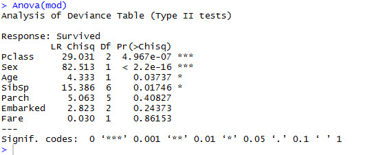
The result shows significance values for only ‘Pclass’, ‘Sex’, ‘Age’, ‘SibSp’ , so we’ll build a second model with just these variables and use that for further analysis.

mod2 <- glm(Survived ~ Pclass + Sex + Age + SibSp ,
        family=binomial(link='logit'),data=traindat)
Anova(mod2)

Let’s visualize the relationships between the response and predictor variables.

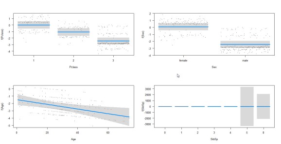
• The log odds (since we used link= ‘logit’) of survival seems to decline as the passenger’s class decreases.
• Women have a higher log odds of survival than men.
• Higher the age gets, lower the log odds of survival get.
• The number of siblings/spouses aboard* also affects the log odds of survival. The log odds for numbers 5 and 8 can go either way indicated by the wide CIs. (*needs to be explored more).

Model Performance:

We will test the peformance of mod2 in predicting ‘Survival’ on a new set of data.

pred <- predict(mod2,newdata=testdat[,-2],type="response")
pred <- ifelse(pred > 0.5,1,0)
testdat$Survived <- as.numeric(levels(testdat$Survived))[testdat$Survived]
rmse <- sqrt((1/nrow(testdat)) * sum( (testdat$Survived - pred) ^ 2))
rmse  #0.4527195

error <- mean(pred != testdat$Survived)
print(paste('Accuracy',1-error)) #81% accuracy

81.171% passenger has been correctly classified.

But when I used the same model to run predictions on Kaggle’s test dataset, the uploaded results fetched me a 75.86 %. I’m guessing the reason could be the arbit split ratio between the ‘traindat’ and ‘testdat’. Maybe next time I’ll employ some sort of bootstrapping.

Well, this is pretty much it for now. I will attempt to better my score in the upcoming weeks (time permitting) and in the event I am successful, I shall add subsequent blog posts and share my learnings (Is that even a word?!).

One thing’s for sure though –  This road is loooooong, is long , is long . . . . .

Later!