
Express dplyr Part II
Want to share your content on R-bloggers? click here if you have a blog, or here if you don't.
This is Part II of the “Express dplyr” posting. If you haven’t already you might want to review Part I of this topic before proceeding although if you have some knowledge of dplyr then by all means proceed. Don’t worry – there are no tests ! In this second part we will work with some “real” data to help solidify our understanding of the dplyr concepts we studied previously. Note that as I wrote this posting I’ve offered up examples I put together very fast which means that there are probably opportunities for improvement and optimization. I want to present examples that can be understood by newcomers to dplyr so I’ve constructed the examples with this in mind.
The Bay Area Bike Share program allows Bay area residents to use bicycles for commuting in the area. Here is a description of the service from the website:
Users of this service can purchase an annual membership online or get a 24-hour or 3-day membership from any station kiosk. 24-hour and 3-day members will receive a ride code from the station kiosk. Enter this code on the keypad next to any available bike. Annual members can bypass the kiosk and insert their membership key at any available dock. Wait for the green light, and pull the bike out while lifting the seat. After your trip, return the bike to any station in your service area. Push the bike firmly into an available dock, and wait for the green light to confirm your trip has ended. Enjoy unlimited trips up to 30 minutes each at no additional cost! Remember, trips longer than 30 minutes will incur overtime fees. 24-hour and 3-day members must request a new ride code for each trip by swiping their credit or debit card at the kiosk
I obtained data relating to this project from the Kaggle Project page. It represents anonymized Bike Data usage from 2013-2015. The data is about 660MB and you can download it though you will need a Kaggle account. The download contains an SQLite Database which is very cool though we’ll ignore that for now and work with the CSV files.
system("unzip -l sf-bay-area-bike-share.zip")
Archive:  sf-bay-area-bike-share.zip
  Length     Date   Time     Name
 --------    ----   ----     ----
2712824832  06-14-16 04:18   database.sqlite
     5647   06-14-16 04:18   station.csv
1989696383  06-14-16 04:18   status.csv
 80208848   06-14-16 04:18   trip.csv
   438063   06-14-16 04:18   weather.csv
 --------                    -------
4783173773                   5 files

# Let's pull out the CSV files of interest

system("unzip sf-bay-area-bike-share.zip station.csv trip.csv weather.csv")
Archive:  sf-bay-area-bike-share.zip
  inflating: station.csv
  inflating: trip.csv
  inflating: weather.csv

library(dplyr)
library(readr)

# Read in the station data
stations <- read_csv("station.csv")

# Read in the trip date - you might get some messages about missing zipcodes
# but don't worry if you do

trips    <- read_csv("trip.csv")

str(stations)

Classes ‘tbl_df’, ‘tbl’ and 'data.frame':	70 obs. of  7 variables:
 $ id               : int  2 3 4 5 6 7 8 9 10 11 ...
 $ name             : chr  "San Jose Diridon Caltrain Station" "San Jose Civic Center" "Santa Clara at Almaden" "Adobe on Almaden" ...
 $ lat              : num  37.3 37.3 37.3 37.3 37.3 ...
 $ long             : num  -122 -122 -122 -122 -122 ...
 $ dock_count       : int  27 15 11 19 15 15 15 15 15 19 ...
 $ city             : chr  "San Jose" "San Jose" "San Jose" "San Jose" ...
 $ installation_date: chr  "8/6/2013" "8/5/2013" "8/6/2013" "8/5/2013" ...

str(trips)

Classes ‘tbl_df’, ‘tbl’ and 'data.frame':	669959 obs. of  11 variables:
 $ id                : int  4576 4607 4130 4251 4299 4927 4500 4563 4760 4258 ...
 $ duration          : int  63 70 71 77 83 103 109 111 113 114 ...
 $ start_date        : chr  "8/29/2013 14:13" "8/29/2013 14:42" "8/29/2013 10:16" "8/29/2013 11:29" ...
 $ start_station_name: chr  "South Van Ness at Market" "San Jose City Hall" "Mountain View City Hall" "San Jose City Hall" ...
 $ start_station_id  : int  66 10 27 10 66 59 4 8 66 10 ...
 $ end_date          : chr  "8/29/2013 14:14" "8/29/2013 14:43" "8/29/2013 10:17" "8/29/2013 11:30" ...
 $ end_station_name  : chr  "South Van Ness at Market" "San Jose City Hall" "Mountain View City Hall" "San Jose City Hall" ...
 $ end_station_id    : int  66 10 27 10 67 59 5 8 66 11 ...
 $ bike_id           : int  520 661 48 26 319 527 679 687 553 107 ...
 $ subscription_type : chr  "Subscriber" "Subscriber" "Subscriber" "Subscriber" ...
 $ zip_code          : int  94127 95138 97214 95060 94103 94109 95112 95112 94103 95060 ...
With regard to the two files above a possible linking key in a join or merge of these two data frames is the id column from stations and perhaps the start_station_id and/or the end_station_id from trips. However, it might not be necessary to join the data just yet as there might be some questions that can be answered by referencing just a single table. In terms of starting to explore the data just begin thinking of some fundamental questions to get the creative juices flowing. Unless you have been given a specific assignment or set of questions there is no “right way” to do something like this. One of the biggest problems I see with students is that if you present them with an open ended opportunity for investigation they freeze up. They had much rather be given a question set and work against that but in the “real world” it isn’t really like that. Just dive in and you will be fine.
Asking Some Questions
How many bikes are there ?
Bikes have a unique identifier and are used any number of times by subscribers. The trips data table has a record of what bike was used in a given trip so we can select that column and then pipe into the distinct() function which will give us a list of all unique bike ids used. This results in a data table whose output we pipe into the nrow() function to count the number of unique bikes used.
trips %>% select(bike_id) %>% distinct()
Source: local data frame [700 x 1]

   bike_id
     (int)
1      520
2      661
3       48
4       26
5      319
6      527
7      679
8      687
9      553
10     107
..     ...

# But if we wanted a single result we could do this

trips %>% select(bike_id) %>% distinct() %>% nrow()
[1] 700

# So how many times was each bike used ?

trips %>% group_by(bike_id) %>% summarize(times_used=n()) %>% arrange(desc(times_used))
Source: local data frame [700 x 2]

   bike_id times_used
     (int)      (int)
1      392       2061
2      489       1975
3      558       1955
4      267       1951
5      631       1948
6      518       1942
7      532       1933
8      592       1932
9      395       1927
10     368       1926
..     ...        ...
I should point out here that dplyr offers a function called count() that will do tallying/counting of data and also accomplish the group_by() and summarize() steps underneath the hood. So when determining the number of times each bike was used consider this:
trips %>% count(bike_id,sort=TRUE)
Source: local data frame [700 x 2]

   bike_id     n
     (int) (int)
1      392  2061
2      489  1975
3      558  1955
4      267  1951
5      631  1948
6      518  1942
7      532  1933
8      592  1932
9      395  1927
10     368  1926
..     ...   ...
Finding Missing Data ?
Since there were some apparent problems when reading in the trips data let’s see if we have a problem with complete cases. I suspect there are missing values in some of the zipe codes. In native R there are some functions like complete.cases() and is.na() and na.omit() that can help you figure out the “missingness” of your data. The following example also gives me an opportunity to explain how dplyr can intersect with native R commands. So we will see that the zip_code column has 17,685 missing values. Note that what I do here is pipe the trips data table into a non dplyr function.
So what columns in the trips data frame contain missing values and if so how many ?
# A pure native R solution
sapply(trips,function(x) sum(is.na(x)))
                id           duration         start_date
                 0                  0                  0
start_station_name   start_station_id           end_date
                 0                  0                  0
  end_station_name     end_station_id            bike_id
                 0                  0                  0
 subscription_type           zip_code
                 0              17685


# A dplyr equivalent

trips %>% sapply(function(x) sum(is.na(x)))
                id           duration         start_date start_station_name
                 0                  0                  0                  0
  start_station_id           end_date   end_station_name     end_station_id
                 0                  0                  0                  0
           bike_id  subscription_type           zip_code
                 0                  0              17685

  subscription_type zip_code
              (int)    (int)
1                 0    17685
So how many cities are covered by the service ? How many stations per city are there ?
stations %>% count(city)
Source: local data frame [5 x 2]

           city     n
          (chr) (int)
1 Mountain View     7
2     Palo Alto     5
3  Redwood City     7
4 San Francisco    35
5      San Jose    16

# We could also sort the result from highest count to lowest

 stations %>% count(city,sort=TRUE)
Source: local data frame [5 x 2]

           city     n
          (chr) (int)
1 San Francisco    35
2      San Jose    16
3 Mountain View     7
4  Redwood City     7
5     Palo Alto     5
Mapping
Here is something cool. We can pipe the locations of the stations to the leaflet package which provides an R interface to the popular Leaflet Javascript library. Once you install the package you can easily map all the stations. The following will produce an interactive map that from a high level will show circles containing numbers that indicate the number of stations in that area. Click on a circle to “drill down” to a more granular level to see where the stations are. If you click on the cluster circle over Palo Alto you will see it split into two clusters of 7 and 5 corresponding to the cities of Redwood City and Palo Alto respectively. The image below is just a screenshot of course but click it to enlarge the map.
library(leaflet)

m <- leaflet() %>% addTiles() %>%
     addMarkers(lng=stations$long,lat=stations$lat,popup=stations$name,
                clusterOptions = markerClusterOptions())

m

LeafLet Cluster Map of Ride Share Stations
Sorting Out The Dates
Note that there is a start_date and end_date for each trip. If we want to do any summary on this information it’s not a bad idea to parse them into an actual date recognized by R. The readr function comes with some date and time routines that we can use here although for more general use the lubridate package is a great package for manipulating dates and times. This can be confusing since native R provides date functions of its own. For now we will use the parse_datetime() function from the readr package.
trips %>% mutate(start_date=parse_datetime(start_date,
                                           format="%m/%d/%Y %H:%M"),
                 end_date=parse_datetime(end_date,
                                           format="%m/%d/%Y %H:%M")) -> trips

# So it looks like the data set starts on August 29, 2013 and continued to
# August 31, 2015

range(trips$start_date)
[1] "2013-08-29 09:08:00 UTC" "2015-08-31 23:26:00 UTC"

trips
Source: local data frame [669,959 x 11]

      id duration          start_date       start_station_name start_station_id            end_date         end_station_name
   (int)    (int)              (time)                    (chr)            (int)              (time)                    (chr)
1   4576       63 2013-08-29 14:13:00 South Van Ness at Market               66 2013-08-29 14:14:00 South Van Ness at Market
2   4607       70 2013-08-29 14:42:00       San Jose City Hall               10 2013-08-29 14:43:00       San Jose City Hall
3   4130       71 2013-08-29 10:16:00  Mountain View City Hall               27 2013-08-29 10:17:00  Mountain View City Hall
4   4251       77 2013-08-29 11:29:00       San Jose City Hall               10 2013-08-29 11:30:00       San Jose City Hall
5   4299       83 2013-08-29 12:02:00 South Van Ness at Market               66 2013-08-29 12:04:00           Market at 10th
6   4927      103 2013-08-29 18:54:00      Golden Gate at Polk               59 2013-08-29 18:56:00      Golden Gate at Polk
7   4500      109 2013-08-29 13:25:00   Santa Clara at Almaden                4 2013-08-29 13:27:00         Adobe on Almaden
8   4563      111 2013-08-29 14:02:00      San Salvador at 1st                8 2013-08-29 14:04:00      San Salvador at 1st
9   4760      113 2013-08-29 17:01:00 South Van Ness at Market               66 2013-08-29 17:03:00 South Van Ness at Market
10  4258      114 2013-08-29 11:33:00       San Jose City Hall               10 2013-08-29 11:35:00              MLK Library
..   ...      ...                 ...                      ...              ...                 ...                      ...
Variables not shown: end_station_id (int), bike_id (int), subscription_type (chr), zip_code (int)
Now should we assume that all trips are started and completed on the same day ? My initial guess is that they are although that might not be true and/or there might have been an error in the data capture. Either way it’s probably wise to check. Looks like there were 2,099 trips that were started on one day and finished the next.
How many trips did not finish on the same day they began ?
trips %>% filter(substr(start_date,1,10)
                        != substr(end_date,1,10)) %>%
                        summarize(different_days=n())
 different_days
           (int)
1           2099
How many trips were there for each year ?
trips %>% count(substr(start_date,1,4))
Source: local data frame [3 x 2]

  substr(start_date, 1, 4)      n
                     (chr)  (int)
1                     2013 100563
2                     2014 326339
3                     2015 243057
Okay let’s extend this a little bit. We will look at the number of trips for each day of each year and use the googleVis package to create a heatmap to visualize this. We’ll need to modify the start_date to respect only the year and ignore the hour and minute portion. The way we did this above was by using the substr() function. However, the googleVis package expects an actual date as opposed to a character string (which is what gets returned by substr() so we’ll need to work a little bit harder (but not too much). So we use the as.Date() to truncate the full date string into just the Year, Month, and Day. We’ll then filter out just the trips that began and ended on the same day, then group by start date, and then count the number of trips for each day. Remember – we are NOT changing the underlying trips date frame at all – we just use the pipe operator to mutate, filter, group, and summarize the data in a single command chain. There is no need to store temporary or intermediate results into a data frame unless you want to.
library(googleVis)

trips %>% mutate(start_date=as.Date(start_date),
                 end_date=as.Date(end_date)) %>%
                 filter(start_date == end_date) %>%
                 count(start_date) -> tripdates

# Create a Gvisplot and then plot it

plot(
  gvisCalendar(data=tripdates, datevar="start_date", numvar="n",
               options=list(
                 title="Calendar Heat Map of Open Bike Trips",
                 calendar="{cellSize:10,
                 yearLabel:{fontSize:20, color:'#444444'},
                 focusedCellColor:{stroke:'red'}}",
                 width=590, height=320),
               chartid="Calendar")
)
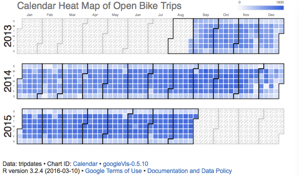
Trips per Day of Year
Trips by Day of the Week
One of the advantages of turning the start and end dates into actual date objects is because we can then use built in R date functions. For example how many trips were there for each day of the week ? We can leverage the strength of the weekdays() function to figure this out.
trips %>% mutate(weekdays = weekdays(start_date)) %>%
         count(weekdays, sort=TRUE)
Source: local data frame [7 x 2]

   weekdays      n
      (chr)  (int)
1   Tuesday 122259
2 Wednesday 120201
3  Thursday 119089
4    Monday 115873
5    Friday 109361
6  Saturday  44785
7    Sunday  38391

# But let's plot this

trips %>% mutate(weekdays = weekdays(start_date)) %>%
  count(weekdays, sort=TRUE) %>%
   ggplot(aes(x=weekdays,y=n)) +
   geom_bar(stat="identity") +
   ggtitle("Trips per Day of The Week") +
   ylab("Total Trips")

Joins
Up until now we have been working with a single table and summaries thereof. Next let’s use our knowledge of joins and merging to learn more about the data. For example, what are the most popular bike stations ? How would we answer this question ? Well we have a list of all the trips in the trips data frame which includes the beginning and ending station id for each trip. So, for each station, is there a way to find the number of trips starting or ending there ? If so then we can find the stations with the highest number of starts and stops which will then tell us the most popular stations.
# For each station we count the number of trips initiated from the
# station or ended there.

# Here we get the number of times a trip started at a station

trips %>% count(start_station_id) -> start

Source: local data frame [70 x 2]

   start_station_id     n
              (int) (int)
1                 2  9558
2                 3  1594
3                 4  3861
4                 5  1257
5                 6  2917
6                 7  2233
7                 8  1692
8                 9  1910
9                10  2393
10               11  2034
..              ...   ...

# Here we get the number of times a trip ended at a station

trips %>% count(end_station_id) -> end

Source: local data frame [70 x 2]

   end_station_id     n
            (int) (int)
1               2  9415
2               3  1786
3               4  3705
4               5  1169
5               6  3163
6               7  2498
7               8  1707
8               9  2200
9              10  1658
10             11  2508
..            ...   ...

# Let's join these two tables using the station_ids as keys. While we do
# the join we can add together the start and end counts for each
# station. This tells us how "popular" a given station was

inner_join(start,end,by=c("start_station_id"="end_station_id")) %>%
    mutate(total_trips=n.x+n.y) %>%
    arrange(desc(total_trips))

Source: local data frame [70 x 4]

   start_station_id cnt.x cnt.y total_trips
              (int) (int) (int)       (int)
1                70 49092 63179      112271
2                69 33742 35117       68859
3                50 32934 33193       66127
4                60 27713 30796       58509
5                61 25837 28529       54366
6                77 24172 28033       52205
7                65 23724 26637       50361
8                74 24838 25025       49863
9                55 26089 23080       49169
10               76 20165 19915       40080
..              ...   ...   ...         ...

# Okay now let's join this with the stations data frame to get some
# more information such as the latitude and longitude

inner_join(start,end,by=c("start_station_id"="end_station_id")) %>%
     mutate(total=n.x+n.y) %>%
     arrange(desc(total)) %>%
     inner_join(stations,c("start_station_id"="id")) %>%
     select(c(1,4:7,9))

Source: local data frame [70 x 6]

   start_station_id total                                          name      lat
              (int)       (int)                                         (chr)    (dbl)
1                70      112271      San Francisco Caltrain (Townsend at 4th) 37.77662
2                69       68859       San Francisco Caltrain 2 (330 Townsend) 37.77660
3                50       66127          Harry Bridges Plaza (Ferry Building) 37.79539
4                60       58509                        Embarcadero at Sansome 37.80477
5                61       54366                               2nd at Townsend 37.78053
6                77       52205                             Market at Sansome 37.78963
7                65       50361                               Townsend at 7th 37.77106
8                74       49863                             Steuart at Market 37.79414
9                55       49169 Temporary Transbay Terminal (Howard at Beale) 37.78976
10               76       40080                                 Market at 4th 37.78630
..              ...         ...                                           ...      ...
Variables not shown: long (dbl), city (chr)
More Mapping
Wouldn’t it be nice to plot this information on a map ? We could plot points representing the station locations and maybe even make the size of a given point/location to be in proportion to the number of trips starting and ending with that given station. This would make it really easy to see which stations get a lot of traffic. To do this we know we are going to need the latitude and longitude information from the stations data frame (but we already have that courtesy of the commands above). Also for purposes of this exercise let’s just focus only on San Francisco bike stations. That is we won’t worry about Palo Alto, Redwood City, Mountain View, or San Jose. Let’s start by reissuing the last command and doing some more selecting to get the right information.
inner_join(start,end,by=c("start_station_id"="end_station_id")) %>%
     mutate(total=n.x+n.y) %>%
     arrange(desc(total)) %>%
     inner_join(stations,c("start_station_id"="id")) %>%
     select(c(1,4:7,9)) %>% filter(city=="San Francisco") -> sfstats

Source: local data frame [35 x 6]

   start_station_id total                                          name      lat      long          city
              (int)       (int)                                         (chr)    (dbl)     (dbl)         (chr)
1                70      112271      San Francisco Caltrain (Townsend at 4th) 37.77662 -122.3953 San Francisco
2                69       68859       San Francisco Caltrain 2 (330 Townsend) 37.77660 -122.3955 San Francisco
3                50       66127          Harry Bridges Plaza (Ferry Building) 37.79539 -122.3942 San Francisco
4                60       58509                        Embarcadero at Sansome 37.80477 -122.4032 San Francisco
5                61       54366                               2nd at Townsend 37.78053 -122.3903 San Francisco
6                77       52205                             Market at Sansome 37.78963 -122.4008 San Francisco
7                65       50361                               Townsend at 7th 37.77106 -122.4027 San Francisco
8                74       49863                             Steuart at Market 37.79414 -122.3944 San Francisco
9                55       49169 Temporary Transbay Terminal (Howard at Beale) 37.78976 -122.3946 San Francisco
10               76       40080                                 Market at 4th 37.78630 -122.4050 San Francisco
..              ...         ...                                           ...      ...       ...           ...

# Next I scale the total number of trips variable down to a reasonable number
# for use with the geom_point function. You could come up with your own
# scaling function to do this. The idea is that when we plot each station
# on the map we can adjust the size of the respective point to reflect how
# busy that station is. There are other ways to do this of course

sz <- round((sfstats$total)^(1/3)-20)

qmap(c(lon=-122.4071,lat=37.78836),zoom=14) -> mymap

mymap +
  geom_point(data=sfstats, aes(x=long,y=lat),
             color="red", alpha=0.4,size=sz) +
             geom_text(data=sfstats,
                       aes(x=long,y=lat,label=start_station_id),size=4)

Plot of SF Stations by Popularity
Two things to note here: 1) the numbers in the circles are the station ids of the associated station. We could have put up the actual station names but that would look messy. 2) There is some over plotting in the lower part of the map because there are two Cal Train related stations very close to each other both of which experience lots of use. So the ids are stacked on top of each other at the current map resolution. We could easily fix this by changing the resolution or plotting these points separately (left as an exercise for the reader).
       San Francisco Caltrain (Townsend at 4th)       49092
        San Francisco Caltrain 2 (330 Townsend)       33742
The “trick” with the sz vector is to find a way to scale the total_trips column in the sfstats data table in a way that let’s us use this figure to specify the size of the point. Here I took the cube root of the total count and subtracted an arbitrary number. I experimented with this but generally find that using root functions can be useful when scaling count data.
What Next ?
We’ve just scratched the surface here. What about identifying the most frequently used trip segments ? We could identify all trip pairs (starting station and ending station id) and count the number of times each occurs. We could then perhaps draw segments on the map to more easily visualize these popular segments. . In a different direction there is another CSV file that came with the data called weather.csv that has meteorological information for each day of the year. We could investigate the impact that weather has on bike usage. Lastly, the data set on Kaggle comes with an SQLite database which we could also use in a couple of ways. dplyr has the ability to connect to SQLite databases though we could also use the RSQLite connection package to execute SQL queries against the database. I’ll explore these options in a future posting. Thanks, Steve Pittard
Filed under: Data Mining, dplyr

R-bloggers.com offers daily e-mail updates about R news and tutorials about learning R and many other topics. Click here if you're looking to post or find an R/data-science job.
Want to share your content on R-bloggers? click here if you have a blog, or here if you don't.