[social4i size=”large” align=”float-right”] Guest post by Khushbu Shah The most common question asked by prospective data scientists is – “What is the best programming language for Machine Learning?” The answer to this question always results in a debate whether to choose R, Python or MATLAB for Machine Learning. Nobody can, in reality, answer the question as to whether Python or R is best language for Machine Learning. However, the programming language one should choose for machine learning directly depends on the requirements of a given data problem, the likes and preferences of the data scientist and the context of machine learning activities they want to perform. According to a survey on Kaggler’s Favourite Tools, the open source R programming language turned out to be the favourite among 543 Kagglers of the 1714 Kaggler’s listing their data science tools. R is the preeminent choice among data professionals who want to understand and explore data, using statistical methods and graphs. It has several machine learning packages and advanced implementations for the top machine learning algorithms – which every data scientist must be familiar with, to explore, model and prototype the given data. R is an open source language to which people have contributed, from around the world. Starting from data collection and cleaning to reproducible research – you will find a Black Box written by someone else, which you can directly use in your program. This Black Box is known as Package in R. A Package in R is nothing but collection of pre-written codes which can be reused. As per CRAN there are around 8,341 packages that are currently available.  Apart from CRAN, there are other repositories which contribute multiple packages. The simple straightforward syntax to install any of these machine learning packages is: install.packages (“Name_Of_R_Package”). Few basic packages without which your life as a data scientist, will be tough include dplyr, ggplot2, reshape2 etc. In this article we will be more focused on packages used in the field of Machine Learning.

Enrol now for a hands-on project based Data Science in R Programming Course

1. MICE Package – Takes care of your Missing Values

   If missing values are something which haunts you then MICE package is the real friend of yours. When we face an issue of missing values we generally go ahead with basic imputations such as replacing with 0, replacing with mean, replacing with mode etc. but each of these methods are not versatile and could result into a possible data discrepancy. MICE package helps you to impute missing values by using multiple techniques, depending on the kind of data you are working with. Let’s take an example on using MICE Package.

       
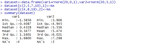
   dataset <- data.frame(var1=rnorm(20,0,1), var2=rnorm(20,5,1))
       dataset[c(2,5,7,10),1] <- NA
       dataset[c(4,8,19),2] <- NA
       summary(dataset)
   

   Till now we have created a random dataframe and introduced few missing values in the data intentionally. Now it’s time to see MICE at work and forget the worry

       install.pckages(“mice”)
       require(mice)
       dataset2 <- mice(dataset)
       dataset2<-complete(dataset2)
       summary(dataset2)

   We have used the default parameters of MICE package for the example, but you can read and change the parameters as per your requirements.

2. rpart package: Lets partition your data

   (rpart) package in R language, is used to build classification or regression models using a two stage procedure and the resultant models is represented in the form of binary trees. The basic way to plot any regression or classification tree using the rpart package is to call the plot() function. The results might not be pretty by just using the basic plot() function, so there is an alternative i.e. the prp() function which is powerful and flexible. prp() function in rpart.plot package is often referred to as the authentic Swiss army knife for plotting regression trees. rpart() function helps establish a relationship between a dependant and independent variables so that a business can understand the variance in the dependant variables based on the independent variables. For instance, if an eLearning company has to find out how their sales (dependant variables) have been impacted due to promotions on Social Media, WOM, Newspapers, Referral Sites, etc. then rpart package has several functions that can help with this analysis phenomenon. rpart stands for Recursive Partitioning and Regression Trees. Using rpart you can run Regression as well as classification. If we talk about syntax, it is pretty simple- rpart(formula, data=, method=,control=)
   • where formula contains the combination of dependent & independent variables; data is the name of your dataset, method depends on the objective i.e. for classification tree, it will beclass; and control is specific to your requirement for example, we want a minimum number variable to split a node etc.
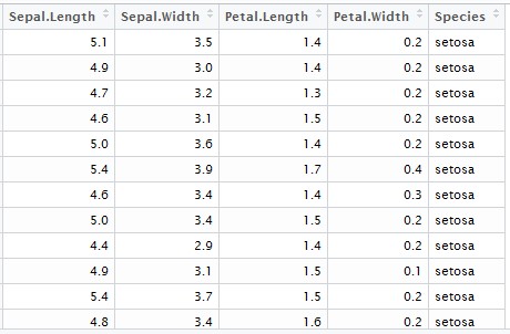
   Let’s consider iris dataset, which looks like - Assuming our objective is to predict Species using a decision tree, it can be achieved by a simple line of code

       rpart_tree <- rpart(formula = Species~., data=iris, method = ‘class’)
       summary(rpart_tree)
       plot(rpart_tree)
   

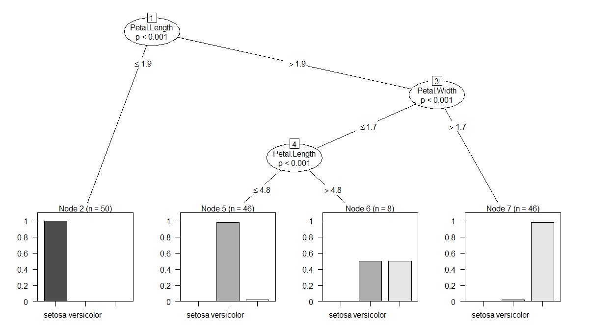
   Let see how does our built tree look like: Here you can see the splits of different nodes and predicted class. To predict for a new dataset, you have simple function predict(tree_name,new_data) which will give you the predicted classes.

3. PARTY: Let’s again partition your data

   PARTY package in R is used for recursive partitioning and this package reflects the continuous development of ensemble methods. PARTY is yet another package to build decision trees based on Conditional Inference algorithm. ctree() is the main function of PARTY package which is used extensively, which reduces the training time and bias. Similar to other predictive analytics functions in R, PARTY also has similar syntax i.e.

   ctree(formula,data)

   which will build your decision tree, taking the default values of various arguments into consideration which can be tweaked based on requirements.

   Let’s build a tree using the same example discussed above.

       party_tree <- ctree(formula=Species~. , data = iris)
       plot(party_tree)
   

   Let see how does the built tree looks like - In this package also you have a predict function which will be used to predict classes for the new data coming in.

4. CARET: Classification And REgression Training

   Classification and REgression Training (CARET) package is developed with the intent to combine model training and prediction. Data scientists can run several different algorithms for a given business problem using the CARET package. Data scientists might not be aware as to which is the best algorithm for a given problem. CARET package helps investigate the optimal parameters for an algorithm with controlled experiments. The grid search method of the caret R package searches parameters by combining various methods to estimate the performance of a given model. After looking at all the trial combinations, the grid search method finds the combination that gives best results. Data scientists can streamline the prices of building predictive models with the help of specialized inbuilt functions for data splitting, feature selection, data pre-processing, variable importance estimation, model tuning through resampling and model visualizations. CARET package is one of the best packages in R. The developers of this package understood that it is hard to know about the best suited algorithm for the given problem case. There can be situations where you are using a particular model and doubting your data but the problem lies in the algorithm you have chosen. After installing CARET package, you can run names(getModelInfo()) and see that there are 217 possible methods which can be run through a single package. To build any predictive model, CARET uses train() function; The syntax of train function looks like – train(formula, data, method) Where method is the predictive model you are trying to build. Let’s use the iris dataset and fit a linear regression model to predict Sepal.Length

       Lm_model <- train(Sepal.Length~Sepal.Width + Petal.Length + Petal.Width, data=iris, method = “lm”)
       summary(lm_model)
   

   CARET package is just not for building models but it also takes care of splitting your data into test and train, do transformation etc. In short, this is the GoTo package in R - for your all Predictive Modeling related needs.

5. randomForest: Let’s combine multiple trees to build our own forest

   Random Forest algorithm is one of the most widely used algorithms when it comes to Machine Learning. R package randomForest is used to create large number of decision trees and then each observation is inputted into the decision tree. The common output obtained for maximum of the observations is considered as the final output. When using randomForest algorithm, data scientists/analysts have to ensure that the variables must be numeric or factors. Factors cannot have more than 32 levels when implementing randomForest. As you must be aware that Random Forest takes random samples of variables as well as observations and build multiple trees. These multiple trees are then combined at the end & votes are taken to finally predict the class of the response variable. Let’s use the iris data example to build a Random Forest using randomForest package. 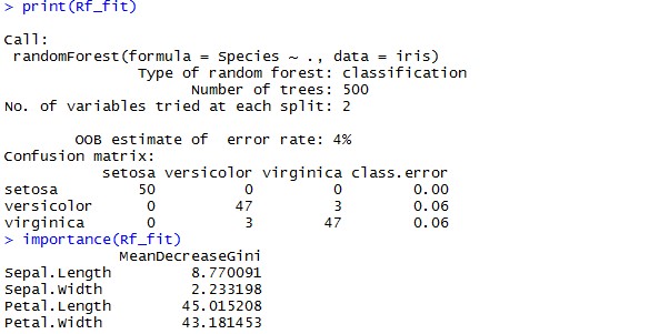Rf_fit<-randomForest(formula=Species~., data=iris) You run a line similar to other packages and your Random Forest is ready to be used. Let see how does this built Forest performs.

       print(Rf_fit)
       importance(Rf_fit)
   

   You might need to play with different control parameters in randomForest e.g., Number of variables in each tree, No. of trees you want to build etc. Generally, data scientists run multiple iterations and select the best combination.

6. nnet: It’s all about hidden layers

   This is the most widely used and easy to understand neural network package, but it is limited to a single layer of nodes. However, several studies have shown that more nodes are not required as they do not contribute in enhancing the performance of the model but rather increase the calculation time and complexity of the model. This package does not provide any specific set of methods for finding the number of nodes in the hidden layer. So, when big data professionals implement nnet it is always suggested that they set it to a value that lies between the number of input and output nodes. nnet packages provides implementation for Artificial Neural Networks algorithm which works - based on the understanding of how a human brain functions, given the input and output signals. ANNs find great applications in forecasting for airlines. In fact, neural network structures provide better forecasts using the nnet functions than the traditional forecasting methods like exponential smoothing, regression, etc. R has multiple packages for building neural networks e.g, nnet, neuralnet, RSNNS. Let’s use our iris data example again (I know you are bored of iris). 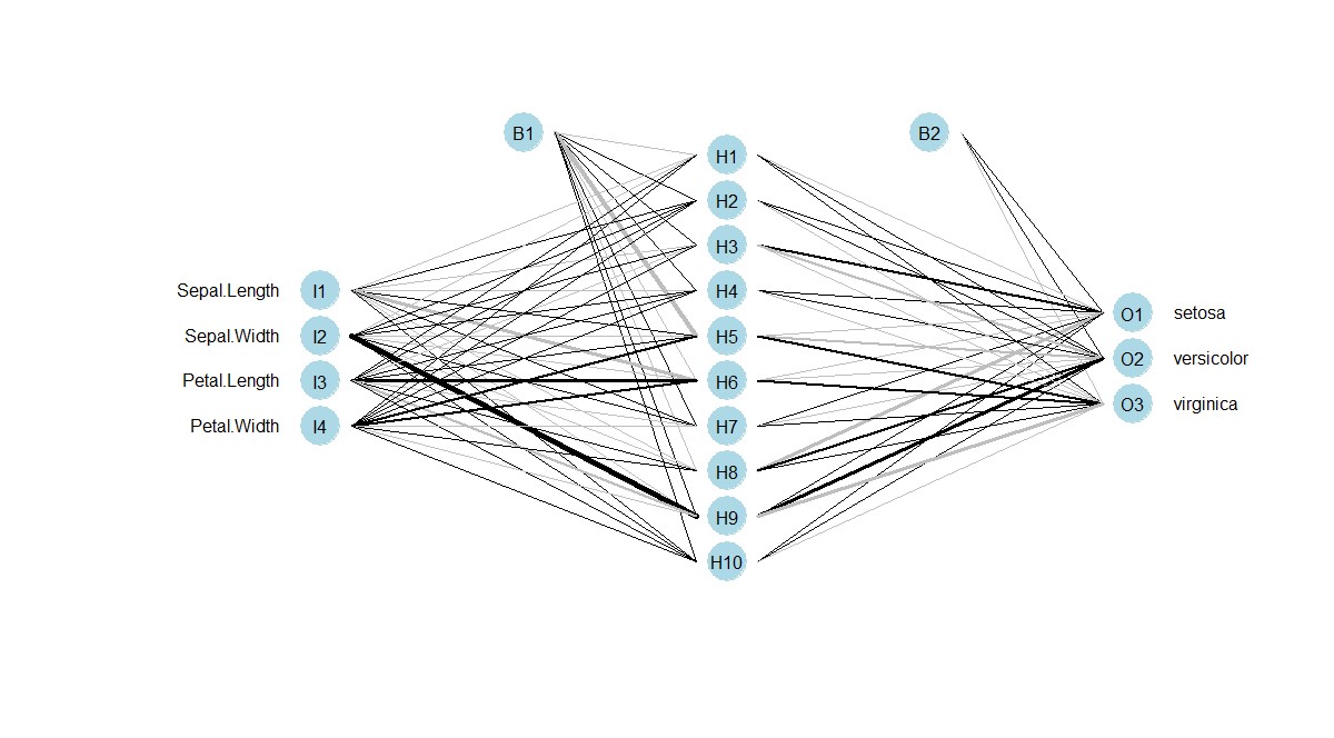Let’s try to predict Species using the nnet now and see how does it look - nnet_model <- nnet(Species~., data=iris, size = 10) You can observe 10 hidden layers in the Neural Network output - this is because we gave size=10 while building the Neural Net. Unfortunately, there is no direct way to plot the built neural networks but there are plenty of custom functions contributed on GitHub which you can use. To build the above shown network we have used - https://gist.githubusercontent.com/fawda123/7471137/raw/466c1474d0a505ff044412703516c34f1a4684a5/nnet_plot_update.r

7. e1071: Let the vectors support your model

   Wondering if this of junk value? Not at all! This is a very vital package in R language that has specialized functions for implementing Naïve Bayes (conditional probability), SVM, Fourier Transforms, Bagged Clustering, Fuzzy Clustering, etc. In fact, the first R interface for SVM implementation was in e1071 R package - for instance, if a data scientist is trying to find out what is the probability that a person who buys an iPhone 6S also buys an iPhone 6S Case. This kind of analysis is based on conditional probability, so data scientists can make use of e1071 R package which has specialized functions for implementing Naive Bayes Classifier. Support Vector Machines are there to rescue you when you have a dataset which is not separable in the given dimensions and you need to promote your data to higher dimensions in order to classify or regress it. Support Vector Machine a.k.a SVM uses Kernel Functions (To optimize mathematical operations) and maximize the margin between two classes. 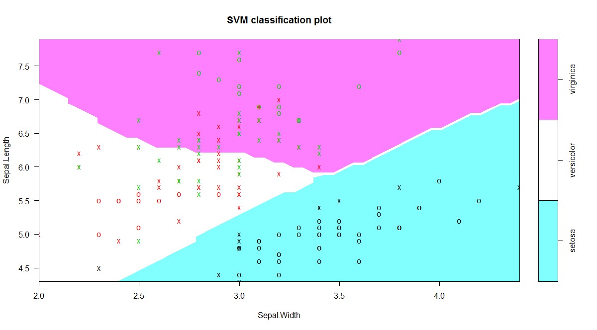Similar to other functions discussed above, syntax for SVM is also similar: svm_model <- svm(Species ~Sepal.Length + Sepal.Width, data=iris) In order to visualize the classified SVM, we need to use plot() function with the data also plot(svm_model, data = iris[,c(1,2,5)]) In the plot shown above, we can clearly see the decision boundaries which were received after applying SVM on iris data. There are multiple parameters which you would have to change in order to get the best accuracy e.g, kernel, cost, gamma, coefficients etc. To get a bet classifier using SVM you will have to experiment with many of these factors, for example kernel can take multiple values like – linear, Gaussian, Cosine etc.

8. kernLab: kernel trick packaged well

   Kernlab takes advantage of the S4 object model in R language, so that data scientists can use kernel based machine learning algorithms. Kernlab has implementations for SVM, kernel feature analysis, dot product primitives, ranking algorithm, Gaussian processes and a spectral clustering algorithm. Kernel based machine learning methods are used when it is challenging to solve clustering, classification and regression problems - in the space in which the observations are made. Kernlab package is widely used in the implementation of SVM which eases pattern recognition to a great extent. It has various kernel functions like – tanhdot (hyperbolic tangent kernel Function), polydot (polynomial kernel function), laplacedot (laplacian kernel function) and many more to perform pattern recognition. Till now you might have understood the power of Kernel functions used in SVM. If Kernel functions are not there, then SVM is not possible altogether. SVM is not the only technique which uses Kernel Trick but there are plenty of other kernel based algorithms which are quite popular and useful, e.g., RVM, Kernel based PCA, Dimensionality reduction etc. kernLab package is a house to ~20 of such algorithms which work on the power of Kernels. kernLab has its own predefined kernels but user has flexibility to build and use their own kernel functions. 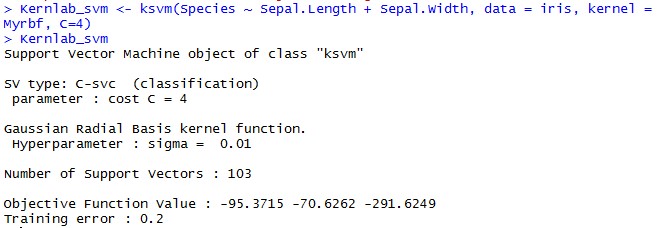Let’s initialize our own Radial Basis Function with a sigma value of 0.01

       Myrbf <- rbfdot(sigma = 0.01)
       Myrbf   
   

   If you want to see the class of Myrbf, you can do it by simply running class() function over the created object Every kernel object accepts two vectors and returns dot product of them. Let’s create two vectors and see their dot products -

       x<-rnorm(10)
       y<-rnorm(10)
       Myrbf(x,y)
   
   
   

   Here we created two random normal variables x & y with 10 values each and computed their dot product using Myrbf kernel. Let’s see an example of SVM using Myrbf kernel We’ll be using iris data again to understand the working of SVM using kernLab -

       Kernlab_svm <- ksvm(Species ~ Sepal.Length + Sepal.Width, data = iris, kernel = Myrbf, C=4)
       Kernlab_svm    
   

   Let’s use the built Support Vector Machine and see how did it predicted:

       predited<-predict(Kernlab_svm,iris)
       table(predicted = predicted, true = iris$Species)
   
   
   
   

Closing Note:

Every package or function in R has some default values associated with it, before applying any algorithm you must know about the various options available. Passing default values will throw you some result but you can’t be sure that the output is the most optimized or accurate one. There are many other machine learning packages available in the CRAN repository like igraph, glmnet, gbm, tree, CORElearn, mboost, etc. which are used in different industries to build performance efficient models. We have observed the scenarios where changing just one parameter can modify the output completely. So, don’t rely on default values of parameters – Understand your data and requirements before applying any algorithm.

Enrol now for a hands-on project based Data Science in R Programming Course