
Intro to The data.table Package
Want to share your content on R-bloggers? click here if you have a blog, or here if you don't.
Data Frames
R provides a helpful data structure called the “data frame” that gives the user an intuitive way to organize, view, and access data. Many of the functions that you would use to read in external files (e.g. read.csv) or connect to databases (RMySQL), will return a data frame structure by default. While there are other important data structures, such as the vector, list and matrix, the data frame winds up being at the heart of many operations not the least of which is aggregation. Before we get into that let me offer a very brief review of data frame concepts:
- A data frame is a set of rows and columns.
- Each row is of the same length and data type
- Every column is of the same length but can be of differing data types
- A data frame has characteristics of both a matrix and a list
- Bracket notation is the customary method of indexing into a data frame
Subsetting Data The Old School Way
Here are some examples of getting specific subsets of information from the built in data frame mtcars. Note that the bracket notation has two dimensions here – one for row and one for column. The comma within any given bracket notation expression separates the two dimensions.
# select rows 1 and 2

mtcars[1:2,]
              mpg cyl disp  hp drat    wt  qsec vs am gear carb
Mazda RX4      21   6  160 110  3.9 2.620 16.46  0  1    4    4
Mazda RX4 Wag  21   6  160 110  3.9 2.875 17.02  0  1    4    4

# select rows 1 and 2 and columns 3 and 5

mtcars[1:2,c(3,5)]
              disp drat
Mazda RX4      160  3.9
Mazda RX4 Wag  160  3.9

# Find the rows where the MPG column is greater than 30

mtcars[mtcars$mpg > 30,]
                mpg cyl disp  hp drat    wt  qsec vs am gear carb
Fiat 128       32.4   4 78.7  66 4.08 2.200 19.47  1  1    4    1
Honda Civic    30.4   4 75.7  52 4.93 1.615 18.52  1  1    4    2
Toyota Corolla 33.9   4 71.1  65 4.22 1.835 19.90  1  1    4    1
Lotus Europa   30.4   4 95.1 113 3.77 1.513 16.90  1  1    5    2

# select columns 10 and 11 for all rows where MPG > 30 and cylinder is
# equal to 4 and then extract columns 10 and 11

mtcars[mtcars$mpg > 30 & mtcars$cyl == 4, 10:11]
               gear carb
Fiat 128          4    1
Honda Civic       4    2
Toyota Corolla    4    1
Lotus Europa      5    2
So the bracket notation winds up being a good way by which to index and search within a data frame although to do aggregation requires us to use other functions such as tapply, aggregate, and table. This isn’t necessarily a bad thing just that you have to learn which function is the most appropriate for the task at hand.
# Get the mean MPG by Transmission

tapply(mtcars$mpg, mtcars$am, mean)
0    1
17.1 24.4

# Get the mean MPG for Transmission grouped by Cylinder

aggregate(mpg~am+cyl,data=mtcars,mean)
   am cyl  mpg
1  0   4 22.9
2  1   4 28.1
3  0   6 19.1
4  1   6 20.6
5  0   8 15.1
6  1   8 15.4

# Cross tabulation based on Transmission and Cylinder

table(transmission=mtcars$am, cylinder=mtcars$cyl)
              cylinder
transmission  4  6  8
0  3  4 12
1  8  3  2
Enter the data.table package
Okay this is nice though wouldn’t it be good to have a way to do aggregation within the bracket notation ? In fact there is. There are a couple of packages that could help us to simplify aggregation though we will start with the data.table package for now. In addition to being able to do aggregation within the brackets there are some other reasons why it is useful:
- It works well with very large data files
- Can behave just like a data frame
-
Offers fast subset, grouping, update, and joins
- Makes it easy to turn an existing data frame into a data table
Since it is an external package you will first need to install it. After that just load it up using the library statement
library(data.table)

dt <- data.table(mtcars)

class(dt)
[1] "data.table" "data.frame"

dt[,mean(mpg)]   # You can't do this with a normal data frame
[1] 20.09062

mtcars[,mean(mpg)]  # Such a thing will not work with regular data frames
Error in mean(mpg) : object 'mpg' not found
So notice that we can actually find the mean MPG directly within the bracket notation. We don’t have to use an external function to do this. So what about reproducing the previous tapply example:
tapply(mtcars$mpg,mtcars$am,mean)
 0    1
17.1 24.4

# Here is how we would do this with the data table "dt"

dt[,mean(mpg),by=am]
   am   V1
1:  1 24.4
2:  0 17.1

# We could even extend this to group by am and cyl

dt[,mean(mpg),by=.(am,cyl)]
    am cyl  V1
1:  1   6 20.6
2:  1   4 28.1
3:  0   6 19.1
4:  0   8 15.0
5:  0   4 22.9
6:  1   8 15.4

# If we want to more clearly label the computed average

dt[,.(avg=mean(mpg)),by=.(am,cyl)]
    am cyl  avg
1:  1   6 20.6
2:  1   4 28.1
3:  0   6 19.1
4:  0   8 15.0
5:  0   4 22.9
6:  1   8 15.4
Similarities to SQL
It doesn’t require many examples to prove that we don’t have to use the aggregate or tapply functions to do any of the work once we have created a data table. Unlike default data frames the bracket notation for a data table object has three dimensions which correspond to what one might see in an SQL statement. Don’t worry – you do not have to be an SQL expert to use data.table. In reality you don’t have to know it at all although if you do then using data.table becomes much easier.

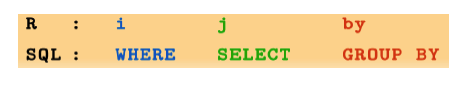
So in terms of SQL we would say something like select “j” (columns or an operation on some columns) where those columns in a row(s) “i” satisfy some specified condition on the rows. And if the “by” index is supplied it indicates how to group the result.
So let’s revisit the previous examples and see how it relates to the SQL model – This is helpful in understanding the paradigm associated with data table objects:
dt[,mean(mpg),by=am]
   am   V1
1:  1 24.4
2:  0 17.1

# The above is analogous to an SQL statement like

select am,avg(mpg) from mtcars group by am

# The following example

dt[,.(avg=mean(mpg)),by=.(am,cyl)]
    am cyl avg
1:  1   6 20.6
2:  1   4 28.1
3:  0   6 19.1
4:  0   8 15.0
5:  0   4 22.9
6:  1   8 15.4

# is analogous to an SQL statement like:

select am,avg(mpg) as avg from mtcars group by am,cyl

# The following example

dt[mpg > 20,.(avg=mean(mpg)),by=.(am,cyl)]
    am cyl  avg
1:  1   6 21.0
2:  1   4 28.1
3:  0   6 21.4
4:  0   4 22.9

# would be analogous to the following SQL statement

select am,avg(mpg) as avg from mtcars where mpg > 20 group by am,cyl
As previously mentioned one does not need to know SQL to use data.table. However, if you do it can help you understand some of the motivations behind the package.
Tabulation
Here are some more examples that illustrate how we can count and tabulate things. Within a data table the special variable .N represents the count of rows. If there is a group by index then it presents the number of rows within that grouping variable.
dt[, .N] # How many rows
[1] 32

dt[, .N, by=cyl]  # How many cars in each cylinder group
   cyl  N
1:   6  7
2:   4 11
3:   8 14

# For rows where the wt is > 1.5 tons count the number of cars by
# transmission type.

dt[wt > 1.5, .(count=.N), by=am]
   am count
1:  1    13
2:  0    19
We can also do sorting quite easily and very fast.
# Present the 5 cars with the best MPG

head(dt[order(-mpg)],5)
 mpg cyl disp  hp drat   wt qsec vs am gear carb
1: 33.9   4 71.1  65 4.22 1.83 19.9  1  1    4    1
2: 32.4   4 78.7  66 4.08 2.20 19.5  1  1    4    1
3: 30.4   4 75.7  52 4.93 1.61 18.5  1  1    4    2
4: 30.4   4 95.1 113 3.77 1.51 16.9  1  1    5    2
5: 27.3   4 79.0  66 4.08 1.94 18.9  1  1    4    1

# Since data table inherits from a data frame we could have also done

dt[order(-mpg)][1:5]
mpg cyl disp  hp drat   wt qsec vs am gear carb
1: 33.9   4 71.1  65 4.22 1.83 19.9  1  1    4    1
2: 32.4   4 78.7  66 4.08 2.20 19.5  1  1    4    1
3: 30.4   4 75.7  52 4.93 1.61 18.5  1  1    4    2
4: 30.4   4 95.1 113 3.77 1.51 16.9  1  1    5    2
5: 27.3   4 79.0  66 4.08 1.94 18.9  1  1    4    1

# We could sort on multiple keys. Here we find the cars with the best
# gas mileage and then sort those on increasing weight

dt[order(-mpg,wt)][1:5]
   mpg cyl disp  hp drat   wt qsec vs am gear carb
1: 33.9   4 71.1  65 4.22 1.83 19.9  1  1    4    1
2: 32.4   4 78.7  66 4.08 2.20 19.5  1  1    4    1
3: 30.4   4 95.1 113 3.77 1.51 16.9  1  1    5    2
4: 30.4   4 75.7  52 4.93 1.61 18.5  1  1    4    2
5: 27.3   4 79.0  66 4.08 1.94 18.9  1  1    4    1
Chicago Crime Statistics
Let’s look at a more realistic example. I have a file that relates to Chicago crime data that you can download if you wish (that is if you want to work this example). It is about 81 megabytes so it isn’t terribly large.
url <- "http://steviep42.bitbucket.org/YOUTUBE.DIR/chi_crimes.csv"
download.file(url,"chi_crimes.csv")
So you might try reading it in with the typical import functions in R such as read.csv which many people use as a default when reading in CSV files. I’m reading this file in on a five year old Mac Book with about 8 GB of RAM. Your speed may vary. We’ll first read in the file using read.csv and then use the fread function supplied by data.table to see if there is any appreciable difference
system.time(df.crimes <- read.csv("chi_crimes.csv", header=TRUE,sep=","))

user system elapsed
30.251 0.283 30.569

nrow(df.crimes)
[1] 334141

# Now let's try fread

system.time(dt.crimes <- fread("chi_crimes.csv", header=TRUE,sep=","))

user system elapsed
1.045 0.037 1.362

attributes(dt.crimes)$class # dt.crimes is also a data.frame
[1] "data.table" "data.frame"

nrow(df.crimes)
[1] 334141

dt.crimes[,.N]
[1] 334141
That was a fairly significant difference. If the file were much larger we would see an even larger difference which for me is a good thing since I routinely read in large files hence fread has become a default for me even if I don’t wind up using the aggregation capability of the data.table package. Also note that the fread function returns a data.table object by default. Now let’s investigate some crime using some of the things we learned earlier.
This data table has information on every call to the Chicago police in the year
2013. So we’ll want to see what factors there are in the data frame/table so we can do
some summaries across groups.
 names(dt.crimes)
 [1] "Case Number"          "ID"                   "Date"
[4] "Block"                "IUCR"                 "Primary Type"
[7] "Description"          "Location Description" "Arrest"
[10] "Domestic"             "Beat"                 "District"
[13] "Ward"                 "FBI Code"             "X Coordinate"
[16] "Community Area"       "Y Coordinate"         "Year"
[19] "Latitude"             "Updated On"           "Longitude"
[22] "Location"

# Let's see how many unique values there are for each column. Looks
# like 30 FBI codes so maybe we could see the number of calls per FBI
# code. What about District ? There are 25 of those.

sapply(dt.crimes,function(x) length(unique(x)))

Case Number                   ID                 Date
334114               334139               121484
Block                 IUCR         Primary Type
28383                  358                   30
Description Location Description               Arrest
296                  120                    2
Domestic                 Beat             District
2                  302                   25
Ward             FBI Code         X Coordinate
51                   30                60704
Community Area         Y Coordinate                 Year
79                89895                    1
Latitude           Updated On            Longitude
180396                 1311               180393
Location
178534
So how many calls per District were there ? Let’s then order this result such that we see the Districts with the highest number of calls first and in descending order.
dt.crimes[,.N,by=District][order(-N)]
1:        8 22386
2:       11 21798
3:        7 20150
4:        4 19789
5:       25 19658
6:        6 19232
7:        3 17649
8:        9 16656
9:       19 15608
10:        5 15258
11:       10 15016
12:       15 14385
13:       18 14178
14:        2 13448
15:       14 12537
16:        1 12107
17:       16 10753
18:       22 10745
19:       17  9673
20:       24  9498
21:       12  8774
22:       13  7084
23:       20  5674
24:       NA  2079
25:       31     6
District     N
Next let’s randomly sample 500 rows and then find the mean number of calls to the cops
as grouped by FBI.Code (whatever that corresponds to) check https://www2.fbi.gov/ucr/nibrs/manuals/v1all.pdf to see them all.
dt.crimes[sample(1:.N,500), .(mean=mean(.N)), by="FBI Code"]
  FBI Code mean
1:       14   60
2:       19    3
3:       24    6
4:       26   47
5:       06  109
6:      08B   83
7:       07   27
8:      08A   22
9:       05   34
10:       18   44
11:      04B   10
12:       03   19
13:       11   15
14:      04A    7
15:       09    1
16:       15    6
17:       16    3
18:       10    1
19:       17    1
20:       02    2
Other Things
Keep in mind that data.table isn’t just for aggregation. You can do anything with it that you can do with a normal data frame. This includes creating new columns, modify existing ones, and create your own functions to do aggregation, and many other activities.
# Get the next to the last row from the data table

dt[.N-1]
mpg cyl disp  hp drat   wt qsec vs am gear carb
1:  15   8  301 335 3.54 3.57 14.6  0  1    5    8

dt[cyl %in% c(4,6)]
mpg cyl  disp  hp drat   wt qsec vs am gear carb
1: 21.0   6 160.0 110 3.90 2.62 16.5  0  1    4    4
2: 21.0   6 160.0 110 3.90 2.88 17.0  0  1    4    4
3: 22.8   4 108.0  93 3.85 2.32 18.6  1  1    4    1
4: 21.4   6 258.0 110 3.08 3.21 19.4  1  0    3    1
5: 18.1   6 225.0 105 2.76 3.46 20.2  1  0    3    1
6: 24.4   4 146.7  62 3.69 3.19 20.0  1  0    4    2
7: 22.8   4 140.8  95 3.92 3.15 22.9  1  0    4    2
8: 19.2   6 167.6 123 3.92 3.44 18.3  1  0    4    4
9: 17.8   6 167.6 123 3.92 3.44 18.9  1  0    4    4
10: 32.4   4  78.7  66 4.08 2.20 19.5  1  1    4    1
11: 30.4   4  75.7  52 4.93 1.61 18.5  1  1    4    2
12: 33.9   4  71.1  65 4.22 1.83 19.9  1  1    4    1
13: 21.5   4 120.1  97 3.70 2.46 20.0  1  0    3    1
14: 27.3   4  79.0  66 4.08 1.94 18.9  1  1    4    1
15: 26.0   4 120.3  91 4.43 2.14 16.7  0  1    5    2
16: 30.4   4  95.1 113 3.77 1.51 16.9  1  1    5    2
17: 19.7   6 145.0 175 3.62 2.77 15.5  0  1    5    6
18: 21.4   4 121.0 109 4.11 2.78 18.6  1  1    4    2

# Summarize different variables at once

dt[,.(avg_mpg=mean(mpg),avg_wt=mean(wt))]
avg_mpg avg_wt
1:    20.1   3.22

dt[,cyl:=NULL]  # Removes the cyl column

head(dt)
mpg disp  hp drat   wt qsec vs am gear carb
1: 21.0  160 110 3.90 2.62 16.5  0  1    4    4
2: 21.0  160 110 3.90 2.88 17.0  0  1    4    4
3: 22.8  108  93 3.85 2.32 18.6  1  1    4    1
4: 21.4  258 110 3.08 3.21 19.4  1  0    3    1
5: 18.7  360 175 3.15 3.44 17.0  0  0    3    2
6: 18.1  225 105 2.76 3.46 20.2  1  0    3    1
Before we finish this posting it is worth mentioning that the data table package also provides support for setting a key much in the same way one would create an index in a relational database to speed up queries. This is for situations wherein you might have a really large data table and expect to routinely interrogate it using the same column(s) as keys. In the next posting I will look at the dplyr package to show another way to handle large files and accomplish intuitive aggregation. Some R experts represents data.table as being as competitor of dplyr although one could mix the two. What I like about data.table is that it allows you to build sophisticated queries, summaries, and aggregations within the bracket notations. It has the added flexibility of allowing you to employ existing R functions or any that you decide to write.
Filed under: data.table, Performance, R programming apply lapply tapply

R-bloggers.com offers daily e-mail updates about R news and tutorials about learning R and many other topics. Click here if you're looking to post or find an R/data-science job.
Want to share your content on R-bloggers? click here if you have a blog, or here if you don't.