
Creating good looking survival curves – the ‘ggsurv’ function
Want to share your content on R-bloggers? click here if you have a blog, or here if you don't.
This is a guest post by Edwin Thoen
Currently I am doing my master thesis on multi-state models. Survival analysis was my favourite course in the masters program, partly because of the great survival package which is maintained by Terry Therneau. The only thing I am not so keen on are the default plots created by this package, by using plot.survfit. Although the plots are very easy to produce, they are not that attractive (as are most R default plots) and legends has to be added manually. I come across them all the time in the literature and wondered whether there was a better way to display survival. Since I was getting the grips of ggplot2 recently I decided to write my own function, with the same functionality as plot.survfitbut with a result that is much better looking. I stuck to the defaults of plot.survfit as much as possible, for instance by default plotting confidence intervals for single-stratum survival curves, but not for multi-stratum curves. Below you’ll find the code of the ggsurv function. Just as plot.survfit it only requires a fitted survival object to produce a default plot. We’ll use the lung data set from the survival package for illustration. First we load in the function to the console (see at the end of this post).
Once the function is loaded, we can get going, we use the lung data set from the survival package for illustration.
library(survival) data(lung) lung.surv <- survfit(Surv(time,status) ~ 1, data = lung) ggsurv(lung.surv) |

Censored observations are denoted by red crosses, by default a confidence interval is plotted and the axes are labeled. Everything can be easily adjusted by setting the function parameters. Now lets look at differences in survival between men and women, creating a multi-stratum survival curve.
lung.surv2 <- survfit(Surv(time,status) ~ sex, data = lung) (pl2 <- ggsurv(lung.surv2)) |
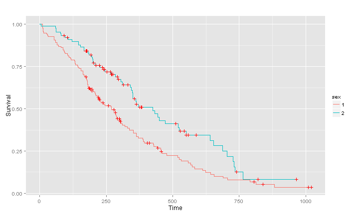
The multi-stratum curves are by default of different colors, the standard ggplot colours. You can set them to your favourite color of course. As always with ggplots a legend is created by default. However we note that levels of the variable sex are called 1 and 2, not very informative. Fortunately the output of ggsurv can still be modified by adding layers after using the function, it is just an ordinary ggplot object.
(pl2 <- pl2 + guides(linetype = F) +
scale_colour_discrete(name = 'Sex', breaks = c(1,2), labels=c('Male', 'Female'))) |

That’s better. Note that the function had also created a legend for linetype, that was non-informative in this case because the linetypes are the same. We removed the legend for linetype before adjusting the one for color.
Finally we can also adjust the plot itself. Maybe the oncologist is very interested in median survival of men and women. Lets help her by showing this on the plot.
lung.surv2
med.surv <- data.frame(time = c(270,270, 426,426), quant = c(.5,0,.5,0),
                       sex = c('M', 'M', 'F', 'F'))
pl2 + geom_line(data = med.surv, aes(time, quant, group = sex),
      col = 'darkblue', linetype = 3) +
geom_point(data = med.surv, aes(time, quant, group =sex), col = 'darkblue') |

I hope survival researchers will take the effort to produce better looking plots after reading this post, although copy pasting the code won’t be too much of an effort I guess.
ggsurv <- function(s, CI = 'def', plot.cens = T, surv.col = 'gg.def',
                   cens.col = 'red', lty.est = 1, lty.ci = 2,
                   cens.shape = 3, back.white = F, xlab = 'Time',
                   ylab = 'Survival', main = ''){

  library(ggplot2)
  strata <- ifelse(is.null(s$strata) ==T, 1, length(s$strata))
  stopifnot(length(surv.col) == 1 | length(surv.col) == strata)
  stopifnot(length(lty.est) == 1 | length(lty.est) == strata)

  ggsurv.s <- function(s, CI = 'def', plot.cens = T, surv.col = 'gg.def',
                       cens.col = 'red', lty.est = 1, lty.ci = 2,
                       cens.shape = 3, back.white = F, xlab = 'Time',
                       ylab = 'Survival', main = ''){

    dat <- data.frame(time = c(0, s$time),
                      surv = c(1, s$surv),
                      up = c(1, s$upper),
                      low = c(1, s$lower),
                      cens = c(0, s$n.censor))
    dat.cens <- subset(dat, cens != 0)

    col <- ifelse(surv.col == 'gg.def', 'black', surv.col)

    pl <- ggplot(dat, aes(x = time, y = surv)) +
      xlab(xlab) + ylab(ylab) + ggtitle(main) +
      geom_step(col = col, lty = lty.est)

    pl <- if(CI == T | CI == 'def') {
      pl + geom_step(aes(y = up), color = col, lty = lty.ci) +
        geom_step(aes(y = low), color = col, lty = lty.ci)
    } else (pl)

    pl <- if(plot.cens == T & length(dat.cens) > 0){
      pl + geom_point(data = dat.cens, aes(y = surv), shape = cens.shape,
                       col = cens.col)
    } else if (plot.cens == T & length(dat.cens) == 0){
      stop ('There are no censored observations')
    } else(pl)

    pl <- if(back.white == T) {pl + theme_bw()
    } else (pl)
    pl
  }

  ggsurv.m <- function(s, CI = 'def', plot.cens = T, surv.col = 'gg.def',
                       cens.col = 'red', lty.est = 1, lty.ci = 2,
                       cens.shape = 3, back.white = F, xlab = 'Time',
                       ylab = 'Survival', main = '') {
    n <- s$strata

    groups <- factor(unlist(strsplit(names
                                     (s$strata), '='))[seq(2, 2*strata, by = 2)])
    gr.name <-  unlist(strsplit(names(s$strata), '='))[1]
    gr.df <- vector('list', strata)
    ind <- vector('list', strata)
    n.ind <- c(0,n); n.ind <- cumsum(n.ind)
    for(i in 1:strata) ind[[i]] <- (n.ind[i]+1):n.ind[i+1]

    for(i in 1:strata){
      gr.df[[i]] <- data.frame(
        time = c(0, s$time[ ind[[i]] ]),
        surv = c(1, s$surv[ ind[[i]] ]),
        up = c(1, s$upper[ ind[[i]] ]),
        low = c(1, s$lower[ ind[[i]] ]),
        cens = c(0, s$n.censor[ ind[[i]] ]),
        group = rep(groups[i], n[i] + 1))
    }

    dat <- do.call(rbind, gr.df)
    dat.cens <- subset(dat, cens != 0)

    pl <- ggplot(dat, aes(x = time, y = surv, group = group)) +
      xlab(xlab) + ylab(ylab) + ggtitle(main) +
      geom_step(aes(col = group, lty = group))

    col <- if(length(surv.col == 1)){
      scale_colour_manual(name = gr.name, values = rep(surv.col, strata))
    } else{
      scale_colour_manual(name = gr.name, values = surv.col)
    }

    pl <- if(surv.col[1] != 'gg.def'){
      pl + col
    } else {pl + scale_colour_discrete(name = gr.name)}

    line <- if(length(lty.est) == 1){
      scale_linetype_manual(name = gr.name, values = rep(lty.est, strata))
    } else {scale_linetype_manual(name = gr.name, values = lty.est)}

    pl <- pl + line

    pl <- if(CI == T) {
      if(length(surv.col) > 1 && length(lty.est) > 1){
        stop('Either surv.col or lty.est should be of length 1 in order
             to plot 95% CI with multiple strata')
      }else if((length(surv.col) > 1 | surv.col == 'gg.def')[1]){
        pl + geom_step(aes(y = up, color = group), lty = lty.ci) +
          geom_step(aes(y = low, color = group), lty = lty.ci)
      } else{pl +  geom_step(aes(y = up, lty = group), col = surv.col) +
               geom_step(aes(y = low,lty = group), col = surv.col)}
    } else {pl}


    pl <- if(plot.cens == T & length(dat.cens) > 0){
      pl + geom_point(data = dat.cens, aes(y = surv), shape = cens.shape,
                      col = cens.col)
    } else if (plot.cens == T & length(dat.cens) == 0){
      stop ('There are no censored observations')
    } else(pl)

    pl <- if(back.white == T) {pl + theme_bw()
    } else (pl)
    pl
  }
  pl <- if(strata == 1) {ggsurv.s(s, CI , plot.cens, surv.col ,
                                  cens.col, lty.est, lty.ci,
                                  cens.shape, back.white, xlab,
                                  ylab, main)
  } else {ggsurv.m(s, CI, plot.cens, surv.col ,
                   cens.col, lty.est, lty.ci,
                   cens.shape, back.white, xlab,
                   ylab, main)}
  pl
} |
R-bloggers.com offers daily e-mail updates about R news and tutorials about learning R and many other topics. Click here if you're looking to post or find an R/data-science job.
Want to share your content on R-bloggers? click here if you have a blog, or here if you don't.