
Unsupervised Google Maps image classification
Want to share your content on R-bloggers? click here if you have a blog, or here if you don't.
This is a guest post by Florian Detsch
Prerequisites
Required packages
First, we need to (install and) load some packages required for data processing and visualization. The below code is mainly based on the Rsenal package, which is a steadily developing, unofficial R library maintained by the Environmental Informatics working group at Philipps-Universität Marburg, Germany. It is hosted on GitHub and features a couple of functions to prepare true-color (satellite) imagery for unsupervised image classification.
# library(devtools)
# install_github("environmentalinformatics-marburg/Rsenal")

lib <- c("Rsenal", "cluster", "rasterVis", "RColorBrewer")
jnk <- sapply(lib, function(x) library(x, character.only = TRUE))
Focal matrices
## 3-by-3 focal matrix (incl. center)
mat_w3by3 <- matrix(c(1, 1, 1,
                      1, 1, 1,
                      1, 1, 1), nc = 3)

## 5-by-5 focal matrix (excl. center)
mat_w5by5 <- matrix(c(1, 1, 1, 1, 1,
                      1, 1, 1, 1, 1,
                      1, 1, 0, 1, 1,
                      1, 1, 1, 1, 1,
                      1, 1, 1, 1, 1), nc = 5)
Google Maps imagery
Rsenal features a built-in dataset (data(gmap_hel)) that shall serve as a basis for our unsupervised classification approach. The image is originated from Google Maps and has been downloaded via dismo::gmap. We previously employed OpenStreetMap::openmap to retrieve BING satellite images of the area. However, massive cloud obscuration prevented any further processing. As seen from the Google Maps image shown below, the land surface is dominated by small to medium-sized shrubs (medium brown) with smaller proportions of tall bushes (dark brown) and bare soil (light brown). Also included are shadows (dark brown to black), which are typically located next to tall vegetation.
data(gmap_hel, package = "Rsenal")
plotRGB(gmap_hel)

Additional input layers
To gather further information on the structural properties of the land surface, a number of artificial layers is calculated from the red, green and blue input bands including
- focal means and standard deviations,
- a visible vegetation index and
- a shadow mask.
5-by-5 focal mean per band
gmap_hel_fcmu <- lapply(1:nlayers(gmap_hel), function(i) {
  focal(gmap_hel[[i]], w = mat_w5by5, fun = mean, na.rm = TRUE, pad = TRUE)
})
gmap_hel_fcmu <- stack(gmap_hel_fcmu)
5-by-5 focal standard deviation per band
gmap_hel_fcsd <- lapply(1:nlayers(gmap_hel), function(i) {
  focal(gmap_hel[[i]], w = mat_w5by5, fun = sd, na.rm = TRUE, pad = TRUE)
})
gmap_hel_fcsd <- stack(gmap_hel_fcsd)
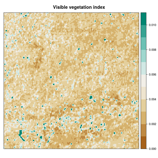
Visible vegetation index
In addition to focal means and standard deviations, we calculate a so-called visible vegetation index (VVI), thus taking advantage of the spectral properties of vegetation in the visible spectrum of light to distinguish between vegetated and non-vegetated surfaces. The VVI is included in Rsenal (vvi) and mainly originates from the red and green input bands.
gmap_hel_vvi <- vvi(gmap_hel)
Shadow mask
We finally create a shadow mask to distinguish between shadow and non-shadow pixels during post-classification image processing. The algorithm is based on the YCbCr color space and is applied to each of the 3 visible bands in a slightly modified form. For further details, the reader is kindly referred to the original article by Deb and Suny (2014). Briefly, the algorithm incorporates a transformation step of the initial RGB raster stack to the YCbCr color space followed by an iterative threshold calculation to distinguish between shadow and non-shadow pixels. Both the color space transformation (rgb2YCbCr) and the subsequent shadow mask algorithm (rgbShadowMask) are included in Rsenal. To get rid of noise (i.e. isolated shadow pixels), we additionally apply a 3-by-3 modal value filter after the actual shadow detection algorithm.
## shadow detection
gmap_hel_shw <- rgbShadowMask(gmap_hel)

## modal filter
gmap_hel_shw <- focal(gmap_hel_shw, w = mat_w3by3,
                      fun = modal, na.rm = TRUE, pad = TRUE)
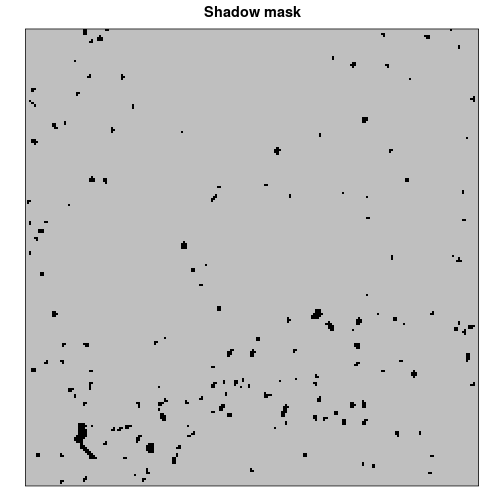
Image classification via kmeans()
The unsupervised image classification is finally realized via kmeans clustering following a nice tutorial by Devries, Verbesselt and Dutrieux (2015). We focus on separating the 3 major land-cover types depicted above, namely
- bare soil (class 'A'),
- small to medium-sized vegetation (class 'B') and
- tall vegetation (class 'C').
## assemble relevant raster data
gmap_hel_all <- stack(gmap_hel, gmap_hel_fcmu, gmap_hel_fcsd, gmap_hel_vvi)

## convert to matrix
mat_hel_all <- as.matrix(gmap_hel_all)

## k-means clustering with 3 target groups
kmn_hel_all <- kmeans(mat_hel_all, centers = 3, iter.max = 100, nstart = 10)
After inserting the classification results into a separate raster template (rst_tmp), an additional class for shadow (tagged '0') is created through multiplication with the initially created shadow mask.
## raster template
rst_tmp <- gmap_hel[[1]]

## insert values
rst_tmp[] <- kmn_hel_all$cluster

## apply shadow mask
rst_tmp <- rst_tmp * gmap_hel_shw
The clusters are initialized randomly, and hence, each land-cover type will be assigned a different ID when running the code repeatedly (which renders automated image creation impossible). Consequently, visual inspection of rst_tmp is required to assign classes 'A', 'B' and 'C' to the respective feature IDs of the previously ratified raster. In our case, bare soil is represented by '1', small vegetation by '3', and tall vegetation by '2'. Note that shadow will always be associated with '0' due to multiplication.
rat_tmp <- ratify(rst_tmp)
rat <- rat_tmp@data@attributes[[1]]
rat$Class <- c("S", "C", "A", "B")
rat <- rat[order(rat$Class), , ]
levels(rat_tmp) <- rat
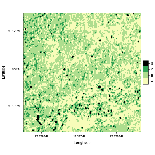
Visualization
Finally, the classified raster can nicely be visualized using the 'YlGn' color palette from COLORBREWER 2.0 along with levelplot from the rasterVis package.
ylgn <- brewer.pal(3, "YlGn")
names(ylgn) <- c("A", "B", "C")
ylgnbl <- c(ylgn, c("S" = "black"))
levelplot(rat_tmp, col.regions = ylgnbl)
R-bloggers.com offers daily e-mail updates about R news and tutorials about learning R and many other topics. Click here if you're looking to post or find an R/data-science job.
Want to share your content on R-bloggers? click here if you have a blog, or here if you don't.