
Understanding Linear SVM with R
Want to share your content on R-bloggers? click here if you have a blog, or here if you don't.
Linear Support Vector Machine or linear-SVM(as it is often abbreviated), is a supervised classifier, generally used in bi-classification problem, that is the problem setting, where there are two classes. Of course it can be extended to multi-class problem. In this work, we will take a mathematical understanding of linear SVM along with R code to understand the critical components of SVM. Taking the liberty to assume that some readers are new to machine learning, let us first find out what the supervised classifier is supposed to do. The term supervised comes from the concept of supervised learning. In case of supervised learning, you provide some examples along with their labels to your classifier and the classifier then tries to learn important features from the provided examples. For example, consider the following data set. You, will provide a part of this data to your linear SVM and tune the parameters such that your SVM can can act as a discriminatory function separating the ham messages from the spam messages. So, let us add the following R-code to our task.
sms_data<-read.csv("sms_spam.csv",stringsAsFactors = FALSE)
head(sms_data)
  type
1  ham
2  ham
3 spam
4  ham
5  ham
6 spam
                                                                                                                                                         text
1                                             Go until jurong point, crazy.. Available only in bugis n great world la e buffet... Cine there got amore wat...
2                                                                                                                               Ok lar... Joking wif u oni...
3 Free entry in 2 a wkly comp to win FA Cup final tkts 21st May 2005. Text FA to 87121 to receive entry question(std txt rate)T&C's apply 08452810075over18's
4                                                                                                           U dun say so early hor... U c already then say...
5                                                                                               Nah I don't think he goes to usf, he lives around here though
6        FreeMsg Hey there darling it's been 3 week's now and no word back! I'd like some fun you up for it still? Tb ok! XxX std chgs to send, £1.50 to rcv
What Parameters should be tuned
Linear SVM tries to find a separating hyper-plane between two classes with maximum gap in-between. A hyper-plane in \(d\)- dimension is a set of points \(x \in \mathbb R^{d}\) satisfying the equation
$$w^{T}x+b=0$$
Let us denote \(h(x)=w^{T}(x)+b\)
Here \(w \) is a \(d\)-dimensional weight vector while \(b\) is a scalar denoting the bias. Both \(w\) and \(b\) are unknown to you. You will try to find and tune both \(w\) and \(b\) such that \(h(x)\) can separate the spams from hams as accurately as possible. I am drawing an arbitrary line to demonstrate a separating hyper-plane using the following code.
plot(c(-1,10), c(-1,10), type = "n", xlab = "x", ylab = "y", asp = 1)
abline(a =12 , b = -5, col=3)
text(1,5, "h(x)=0", col = 2, adj = c(-.1, -.1))
text(2,3, "h(x)>0,Ham", col = 2, adj = c(-.1, -.1))
text(0,3, "h(x)<0,Spam", col = 2, adj = c(-.1, -.1))
This is plot we get:

Oh, btw, did you notice that Linear SVM has decision rules. Let \(y\) be an indicator variable which takes the value -1 if the message is spam and 1 if it is a ham. Then, the decision rules are
$$y=-1~iff~h(x)~is~less~than~0$$
$$y=1~iff~h(x)~is~greater~than~0$$
Notice that for any point \(x\) in your data set, \(h(x)\neq 0\) as we want the function \(w^{T}x+b\) to clearly distinguish between spam and ham. This brings us to a important condition.
Important Condition
Linear SVM assumes that the two classes are linearly separable that is a hyper-plane can separate out the two classes and the data points from the two classes do not get mixed up. Of course this is not an ideal assumption and how we will discuss it later how linear SVM works out the case of non-linear separability. But for a reader with some experience here I pose a question which is like this Linear SVM creates a discriminant function but so does LDA. Yet, both are different classifiers. Why ? (Hint: LDA is based on Bayes Theorem while Linear SVM is based on the concept of margin. In case of LDA, one has to make an assumption on the distribution of the data per class. For a newbie, please ignore the question. We will discuss this point in details in some other post.)
Properties of \(w\)
Consider two points \(a_{1}\) and \(a_{2}\) lying on the hyper-plane defined by \(w^{T}x+b\). Thus, \(h(a_{1})=w^{T}a_{1}+b=0\) and \(h(a_{2})=w^{T}a_{2}+b=0\). Therefore,
$$w^{T}(a_{1}-a_{2})=0$$.
Notice that the vector \(a_{1}-a_{2}\) is lying on the separating hyper-plane defined by \(w^{T}x+b\). Thus, \(w\) is orthogonal to the hyper-plane.
Here it is the plot:

The Role of \(w\)
Consider a point \(x_{i}\) and let \(x_{p}\) be the orthogonal projection of \(x_{i}\) onto the hyper-plane. Assume $h(x_{i})>0$ for \(x\).
\(\frac{w}{\vert\vert w\vert\vert}\) is a unit vector in the direction of \(w\).
Here it is the plot:

Let \(r\) be the distance between \(x_{i}\) and \(x_{p}\). Since \(x_{i}\) is projected on the hyper-plane, there is some loss of information which is calculated as
$$(r=x_{i}-x_{p})$$.
Notice that \(r\) is parallel to the unit vector \(\frac{w}{\vert\vert w\vert\vert}\) and therefore \(r\) can be written as some multiple of \(\frac{w}{\vert\vert w\vert\vert}\). Thus, \(r=c\times \frac{w}{\vert\vert w\vert\vert}\), for some scalar value \(c\). It can be shown that
$$c=\frac{h(x_{i})}{\vert\vert w\vert\vert}$$
Actually, \(c\times \frac{w}{\vert\vert w\vert\vert}\) represents the orthogonal distance of the point \(x_{i}\) from the hyper-plane. Distance has to be positive. \(\frac{w}{\vert\vert w\vert\vert}\) cannot be negative. However, \(c=\frac{h(x)}{\vert\vert w\vert\vert}\). Though, before starting the equations we assumed that \(h(x_{i})\) is positive, but that is not a general case. In general \(c\) can be negative also. Therefore we multiply \(y\) with \(c\). Remember your \(y\) from the decision rules. That is
$$c=y\times \frac{h(x_{i})}{\vert\vert w\vert\vert}$$
The Concept of Margin
Linear SVM is based on the concept of margin which is defined as the smallest value of \(c\) for all the \(n\) points in your training data set. That is
$$\delta^{\star}=min\{c~\forall~points~in~the~training~data~set\}$$. All points \(x^{\star}\) which are lying at an orthogonal distance of \(\delta^{\star}\) from the hyper-plane \(w^{T}x+b=0\) are called support vectors.
Scaling Down the Margin
Let \(\delta^{\star}=\frac{y^{\star}\times h(x^{\star})}{\vert\vert w\vert\vert}\), where \(x^{\star}\) is a support vector. We want \(\delta^{\star} = \frac{1}{\vert\vert w\vert\vert}\). Clearly, we want to multiply some value \(s\) such that \(s\times y^{\star}\times h(x^{\star})=1\). Therefore, \(s=\frac{1}{y^{\star}\times h(x^{\star})}\).
Objective Criteria for Linear SVM
After scaling down, we have the following constraint for SVM:
$$y\times (w^{T}x+b)\geq \frac{1}{\vert\vert w\vert\vert}$$.
Now consider two support vectors, one denoted by \(a_{1}\) on the positive side, while the other \(a_{2}\) on the negative side of the hyper-plane. For the time being let us not use \(y\). Then, we have \(w^{T}a_{1}+b= \frac{1}{\vert\vert w\vert\vert}\) and \(w^{T}a_{2}+b= \frac{-1}{\vert\vert w\vert\vert}\).Thus, \(w^{T}(a_{1}-a_{2})=\frac{2}{\vert\vert w\vert\vert}\).\(w^{T}(a_{1}-a_{2})\) depicts the separation/gap between the support vectors on the either side. We want to maximize this gap \(\frac{2}{\vert\vert w\vert\vert}\). For the purpose, we need to minimize \(\vert\vert w\vert\vert\). Instead,we can minimize \(\frac{\vert\vert w\vert\vert^{2}}{2}\). Formally, we want to solve
$$Minimize_{w,b}\frac{\vert\vert w\vert\vert^{2}}{2}$$
subject to the constraint
$$y_{i}(w^{T}x_{i}+b)\geq \frac{1}{\vert \vert w\vert\vert}~\forall ~x_{i}~in ~Training~Data~set$$.
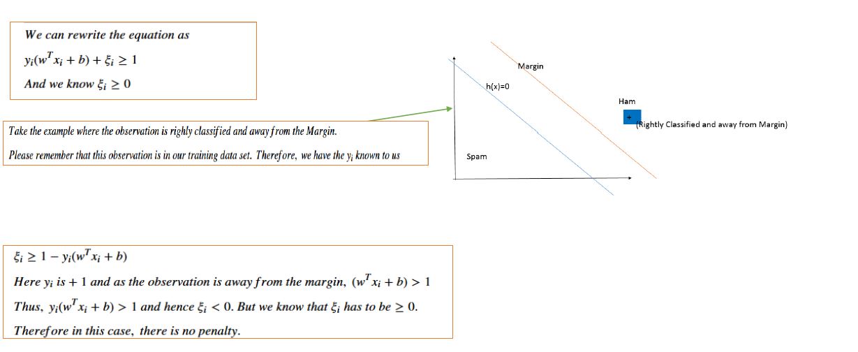
For linearly inseparable case, we introduce some penalty \(0\leq \xi_{i} \leq 1\) in the objective function and our constraint.
$$Minimize_{w,b}(\frac{\vert\vert w\vert\vert^{2}}{2}+ C\sum_{i=1}^{n}\xi_{i})$$
subject to the constraints
$$(1)~y_{i}(w^{T}x_{i}+b)\geq 1-\xi_{i}~\forall ~x_{i}~in ~Training~Data~set~of~size~n$$ and
$$(2)~\xi_{i}\geq 0~\forall ~n~points~in~the~Training~Data~set$$
\(C\) is a user defined parameter.
In case you wish to see how \(\xi_{i}\) is used as penalty, please consider the the three figures below. You can also choose to skip them if the above details are okay for you.


Try the Code with R
Let us now start our coding. The needed code is here.
library(tm)
setwd(path to the directory)
print(getwd())
sms_data<-read.csv("sms_spam.csv",stringsAsFactors = FALSE)

print(head(sms_data))
sms_data$type<-factor(sms_data$type)


simply_text<-Corpus(VectorSource(sms_data$text))

cleaned_corpus<-tm_map(simply_text, tolower)
cleaned_corpus<-tm_map(cleaned_corpus,removeNumbers)
cleaned_corpus<-tm_map(cleaned_corpus,removeWords,stopwords())
#cleaned_corpus<-tm_map(cleaned_corpus,removePunctuation)
#cleaned_corpus<-tm_map(cleaned_corpus,stripWhitespace)

sms_dtm<-DocumentTermMatrix(cleaned_corpus)
sms_train<-sms_dtm[1:4000]
sms_test<-sms_dtm[4001:5574]
#sms_train<-cleaned_corpus[1:4000]
#sms_test<-cleaned_corpus[4001:5574]

freq_term=(findFreqTerms(sms_dtm,lowfreq=2))
#sms_freq_train<-DocumentTermMatrix(sms_train,  list(dictionary=freq_term))
#sms_freq_test<-DocumentTermMatrix(sms_test,list(dictionary=freq_term))

y<-sms_data$type
y_train<-y[1:4000]
y_test<-y[4001:5574]
library(e1071)
tuned_svm<-tune(svm, train.x=sms_freq_train, train.y = y_train,kernel="linear", range=list(cost=10^(-2:2), gamma=c(0.1, 0.25,0.5,0.75,1,2)) )
print(tuned_svm)
adtm.m<-as.matrix(sms_freq_train)
adtm.df<-as.data.frame(adtm.m)
svm_good_model<-svm(y_train~., data=adtm.df, kernel="linear",cost=tuned_svm$best.parameters$cost, gamma=tuned_svm$best.parameters$gamma)

adtm.m_test<-as.matrix(sms_freq_test)
adtm.df_test=as.data.frame(adtm.m_test)
y_pred<-predict(svm_good_model,adtm.df_test)
table(y_test,y_pred)

library(gmodels)
CrossTable(y_pred,y_test,prop.chisq = FALSE)

  type
1  ham
2  ham
3 spam
4  ham
5  ham
6 spam
                                                                                                                                                         text
1                                             Go until jurong point, crazy.. Available only in bugis n great world la e buffet... Cine there got amore wat...
2                                                                                                                               Ok lar... Joking wif u oni...
3 Free entry in 2 a wkly comp to win FA Cup final tkts 21st May 2005. Text FA to 87121 to receive entry question(std txt rate)T&C's apply 08452810075over18's
4                                                                                                           U dun say so early hor... U c already then say...
5                                                                                               Nah I don't think he goes to usf, he lives around here though
6        FreeMsg Hey there darling it's been 3 week's now and no word back! I'd like some fun you up for it still? Tb ok! XxX std chgs to send, £1.50 to rcv

Parameter tuning of ‘svm’:

- sampling method: 10-fold cross validation

- best parameters:
 cost gamma
    1   0.1

- best performance: 0.01825
   Cell Contents
|-------------------------|
|                       N |
|           N / Row Total |
|           N / Col Total |
|         N / Table Total |
|-------------------------|


Total Observations in Table:  1574


             | y_test
      y_pred |       ham |      spam | Row Total |
-------------|-----------|-----------|-----------|
         ham |      1295 |       191 |      1486 |
             |     0.871 |     0.129 |     0.944 |
             |     0.952 |     0.897 |           |
             |     0.823 |     0.121 |           |
-------------|-----------|-----------|-----------|
        spam |        66 |        22 |        88 |
             |     0.750 |     0.250 |     0.056 |
             |     0.048 |     0.103 |           |
             |     0.042 |     0.014 |           |
-------------|-----------|-----------|-----------|
Column Total |      1361 |       213 |      1574 |
             |     0.865 |     0.135 |           |
-------------|-----------|-----------|-----------|
In the above example we are not using the cleaned corpus. We see that the accuracy/precision of our classifier for ham is 0.871 and recall is 0.95. However for Spam messages, the precision is 0.250, while recall is just 0.103. We found that the usage of cleaned corpus degrades the performance for the SVM more.
Related Post
- How to add a background image to ggplot2 graphs
- Streamline your analyses linking R to SAS: the workfloweR experiment
- R Programming – Pitfalls to avoid (Part 1)
- Eclipse – an alternative to RStudio – part 2
- Eclipse – an alternative to RStudio – part 1
R-bloggers.com offers daily e-mail updates about R news and tutorials about learning R and many other topics. Click here if you're looking to post or find an R/data-science job.
Want to share your content on R-bloggers? click here if you have a blog, or here if you don't.