This is probably a slightly useless post, but a bit of fun all the same. If nothing else, it allows me to take a stab at learning a bit more about logistic regression.

I’m still trying to unravel the mystery of why the Bears lost to the Vikings two weeks ago. This mystery is compounded with attempting to understand how the Patriots lost to the Jets in the playoffs in the 2010 season. Very similar stories. Chicago and New England had defeated Minnesota and New York, respectively, several games prior. In the case of the Patriots, they bludgeoned the Jets, allowing only a field goal, while racking up 45 points for themselves.

So what happened? I say that the answer is turnovers. Below, I show a graph of the difference in turnovers for each game the Bears played from 1985 through 2011. I’ve jittered the plots so that the volume of observations is more clear. (This is the part where I note that I took this visual presentation and code from Andrew Gelman and Jennifer Hill’s fantastic book “Data Analysis and Multilevel/Hierarchical Models“. Anything absurd is my doing.)

Note that I calculate turnover difference as the opponent’s turnovers minus Chicago’s turnovers. This way a positive number is a good thing. In other words, if Chicago has 3 turnovers and their opponent has 4, then turnover difference is equal to 1.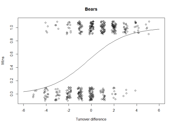
The fit line is a logistic regression of the results. The trend is obvious and shouldn’t surprise anyone with a nodding understanding of football. If you turn the ball over more often than your opponent, it’s more difficult to win a game.

We can use the coefficients of the fit to determine how this affects their (modeled) chance of victory. If the turnover difference is zero, the fit line suggests that the Bears have about a 55% chance of winning (again, this is a fit result over many seasons). If they turn the ball over one more time than their opponent, that probability drops to 40%.

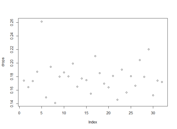
How about other teams? Same story. Analysis of all teams shows a drop of at least 14% and as much as 26% if the turnover difference is -1. (The Ravens are a bit of an outlier, possibly because they’re a newer team. Or because their defense sucks. One or the other.)

The following is a very spartan graph of that point, that I’ll get around to replacing one of these days.

So, how do we predict turnovers? I don’t know.  As I said, this may be a slightly useless post.

Almost forgot the code:

library(XML)
library(lubridate)
library(gtools)

GetTeamSeasonResults = function(year, team)
{

  games.URL.stem = "http://www.pro-football-reference.com/teams/"
  URL = paste(games.URL.stem, team, "/", year, "_games.htm", sep="")

  games = readHTMLTable(URL)

  if (length(games) == 0) {
    return (NULL)
  }

  df = games[[1]]

  df = df[,1:21]

  # Clean up the df
  df[,4] = NULL

  emptyRow = which(df$Tm == "")
  if(length(emptyRow) > 0 )
  {
    df = df[-emptyRow,]
    row.names(df) = seq(nrow(df))
  }

  colnames(df) = c("Week", "Day", "Date", "Outcome", "OT", "Record","Home", "Opponent", "ThisTeamScore", "OpponentScore"
                   , "ThisTeam1D", "ThisTeamTotalYards", "ThisTeamPassYards", "ThisTeamRushYards", "ThisTeamTO"
                   , "Opponent1D", "OpponentTotalYards", "OpponentPassYards", "OpponentRushYards", "OpponentTO")

  df$GameDate = mdy(paste(df$Date, year), quiet=T)
  year(df$GameDate) = with(df, ifelse(month(GameDate) <=6, year(GameDate)+1, year(GameDate)))
  df$Date = as.character(df$Date)
  df$Home = with(df, ifelse(Home == "@",F,T))
  df$TODiff = with(df, as.integer(OpponentTO) - as.integer(ThisTeamTO))
  df$Win = ifelse(df$Outcome =="W", 1, 0)

  return(df)
}

years = 1985:2011
teams = c("nyj",  "mia", "nwe", "buf"
          , "rav", "cin", "pit", "cle"
          , "htx", "clt", "oti", "jax"
          , "den", "sdg", "rai", "kan"
          , "dal", "nyg", "was", "phi"
          , "gnb", "chi", "min", "det"
          , "atl", "tam", "nor", "car"
          , "sfo", "sea", "ram", "crd")

numTeams = length(teams)
teamList = vector("list", numTeams)
for (iTeam in 1:numTeams)
{
  aList = lapply(years, GetTeamSeasonResults, teams[iTeam])
  df = do.call("rbind", aList)
  teamList[[iTeam]] = df
}

rm(aList)

FitTODiff = function(df)
{
  fit = glm(df$Win ~ df$TODiff, family=binomial(link="logit"))
  print(inv.logit (coef(fit)))
  return (fit)
}

fits = lapply(teamList, FitTODiff)

OneGameDrop = function(fit)
{
  drop = inv.logit( coef(fit)[1]) - inv.logit( coef(fit)[1] -coef(fit)[2] )
  return (drop)
}

drops = sapply(fits, OneGameDrop)

plot (drops)