This is a companion post to the article What’s the ROI of your loan? It depends…, which discusses approaches for calculating the return on a P2P loan. In that article I make an off-hand remark about floating point imprecision, which occurred when solving for the internal rate of return (IRR) of a loan. I had a nagging feeling that there was more to the story than that, and indeed there is. It turns out that the behavior is not due to floating point approximations but strictly by the tolerance argument in the uniroot function. This post looks at the effect that tolerance has on precision.

First, let’s set the stage by providing some functions to compute the IRR. Recall that the IRR is defined as the interest rate that makes the present value of a series of cashflows 0. This is why the uniroot function is used, since we are simply finding the root of a function in terms of the interest rate. Here is a simplified version designed to facilitate the discussion. Notice how vectorization and recycling make this function quite compact.

irr <- function(principal, balance, payment, terms, ...)
{
  f <- function(r) {
    cashflows <- sum(payment / (1+r)^(1:terms))
    end.value <- balance / (1+r)^terms[length(terms)]
    -principal + cashflows + end.value
  }
  uniroot(f, c(-0.99,1), ...)$root
}

Next we’ll define an amortization schedule based on a hypothetical loan. Once we create the schedule, we can iterate over the terms to compute the IRR at each time step as the loan matures. The amortization schedule is computed using the following two functions.

amortize <- function(principal, i.rate, terms) {
  principal * i.rate * (1+i.rate)^terms / ((1 + i.rate)^terms - 1)
}

amortization_schedule <- function(principal, i.rate, terms) {
  payment <- amortize(principal, i.rate, terms)
  f <- function(t) {
    principal * (1 - ((1 + i.rate)^t - 1) / ((1 + i.rate)^terms - 1))
  }
  balance <- sapply(1:terms, f)
  ps <- -diff(c(principal,balance))
  is <- payment - ps
  data.frame(principal=ps, interest=is, balance=balance)
}

The example loan I use has $10,000 principal, a 12% interest rate and a 3 year term, payable monthly. To generate the actual schedule, I converted the interest rate and term to a monthly frequency to match the payment frequency.

schedule <- amortization_schedule(10000,.01,36)
payment <- sum(schedule[1,1:2])
is <- sapply(1:36, 
  function(x) irr(10000, 10000 - sum(schedule[1:x,1]), payment, x))

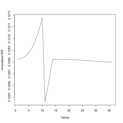
The heartbeat-like spike is an artifact of the root finder based on the mechanics of the tolerance. Verifying this claim is as easy as changing the tolerance of the root finder.

is.5 <- sapply(1:36, 
  function(x) irr(10000, 10000 - sum(schedule[1:x,1]), 
    payment, x, tol=.Machine$double.eps^0.5))

We still see some peaks and valleys, but now the variation in interest rate is less than 1e-7!

Let’s go the other way and look at decreasing the tolerance to .Machine$double.eps^0.125.

is.125 <- sapply(1:36, 
  function(x) irr(10000, 10000 - sum(schedule[1:x,1]), 
    payment, x, tol=.Machine$double.eps^0.125))

The annualized IRR now varies by almost 7 percentage points over the life of the loan!

How can this be? Let’s take a closer look at what tolerance means. Since the machine epsilon is less than one, taking a fractional root is increasing the tolerance. The value of .Machine$double.eps^0.125 is 0.01104854 and half of that is 0.005524272. The peak to valley difference in the heartbeat is diff(range(is.125)) = 0.005028085! So the optimizer is iterating to the closest value, but eventually flips to the lower quantized step once the error is greater than the error in the lower step. It may be difficult to tie this back to the graph, which has annualized values. However, it’s simple to “annualize” the error by applying the same conversion:

> (1 + .Machine$double.eps^.125 / 2)^12 - 1
[1] 0.06834297522498400390134

This explanation misses one important piece, which is why does the IRR drift at all? The answer is that as terms are added, the value at the end points are different. Presumably the steps are taken with respect to the end points, so the change in value will affect where quantization occurs due to the tolerance.

To conclude, numerical analysis requires thinking through the magnitude of the numbers you are working with. You cannot blindly assume that the tolerance is set at an acceptable level. Otherwise, if you are cavalier like me, you may end up with seemingly strange artifacts.