This month’s issue of Significance magazine has a very nice summary article of the sinh-arcsinh normal distribution. (Unfortunately, the article seems to be behind a paywall.)

This distribution was first introduced by Chris Jones and Arthur Pewsey in 2009 as a generalization of the normal distribution. While the normal distribution is symmetric and has light to moderate tails and can be defined by just two parameters ( for location and for scale), the sinh-arcsinh distribution has two more parameters which control asymmetry and tail weight.

Given the 4 parameters, the sinh-arcsinh normal distribution is defined as

where and are the hyperbolic sine function and its inverse.

• controls the location of the distribution (where it is “centered” at),
• controls the scale (the larger it is, the more spread out the distribution is),
• controls the asymmetry of the distribution (can be any real value, more positive means more right skew, more negative means more left skew), and
• controls tail weight (any positive real value,

From the expression, we can also see that when and , the distribution reduces to the normal distribution with mean and standard deviation .

In R, the gamlss.dist package provides functions for plotting this distribution. The package provides functions for 3 different parametrizations of this distribution; the parametrization above corresponds to the SHASHo set of functions. As is usually the case in R, dSHASHo, pSHASHo, qSHASHo and rSHASHo are for the density, distribution function, quantile function and random generation for the distribution.

First, we demonstrate the effect of skewness (i.e. varying ).

library(gamlss.dist)
library(dplyr)
library(ggplot2)

x <- seq(-6, 6, length.out = 301)
nu_list <- -3:3
df <- data.frame()
for (nu in nu_list) {
    temp_df <- data.frame(x = x, 
                          y = dSHASHo2(x, mu = 0, sigma = 1, nu = nu, tau = 1))
    temp_df$nu <- nu
    df <- rbind(df, temp_df)
}

As becomes more positive, the distribution becomes more right-skewed:

df %>% filter(nu >= 0) %>%
    ggplot(aes(x = x, y = y, col = factor(nu))) +
    geom_line() + theme_bw()

As becomes more negative, the distribution becomes more left-skewed:

df %>% filter(nu <= 0) %>%
    ggplot(aes(x = x, y = y, col = factor(nu))) +
    geom_line() + theme_bw()

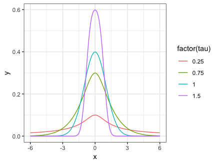
Next, we demonstrate the effect varying has on the weight of the tails. The code and picture below is for when there is no skewness in the distribution:

tau_list <- c(0.25, 0.75, 1, 1.5)
df <- data.frame()
for (tau in tau_list) {
    temp_df <- data.frame(x = x, 
                          y = dSHASHo(x, mu = 0, sigma = 1, nu = 0, tau = tau))
    temp_df$tau <- tau
    df <- rbind(df, temp_df)
}

ggplot(data = df, aes(x = x, y = y, col = factor(tau))) +
    geom_line() + theme_bw()

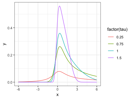
By changing nu = 0 to nu = 1 in the code above, we see the effect of tail weight when there is skewness:

(Note: For reasons unclear to me, the Significance article uses different symbols for the 4 parameters: instead of , instead of , instead of and instead of .)

The authors note that it is possible to perform maximum likelihood estimation with this distribution. It is an example of GAMLSS regression, which can be performed in R using the gamlss package.

References:

1. Jones, C. and Pewsey, A. (2019). The sinh-arcsinh normal distribution.
2. Jones, M. C. and Pewsey, A. (2009). Sinh-arcsinh distributions.