Consider planning a clinicial trial where patients are randomized in permuted blocks of size four to either a ‘control’ or ‘treatment’ group. The outcome is measured on an 11-point ordinal scale (e.g., the numerical rating scale for pain). It may be reasonable to evaluate the results of this trial using a proportional odds cumulative logit model (POCL), that is, if the proportional odds assumption is valid. The POCL model uses a series of ‘intercept’ parameters, denoted $alpha_1 leq ldots leq alpha_{r-1}$, where $r$ is the number of ordered categories, and ‘slope’ parameters $beta_1, ldots, beta_m$, where $m$ is the number of covariates. The intercept parameters encode the ‘baseline’, or control group frequencies of each category, and the slope parameters represent the effects of covariates (e.g., the treatment effect).

A Monte-Carlo simulation can be implemented to study the effects of the control group frequencies, the odds ratio associated with treatment allocation (i.e., the ‘treatment effect’), and sample size on the power or precision associated with a null hypothesis test or confidence interval for the treatment effect.

In order to simulate this process, it’s necessary to specify each of the following:

1. control group frequencies
2. treatment effect
3. sample size
4. testing or confidence interval procedure

Ideally, the control group frequencies would be informed by preliminary data, but expert opinion can also be useful. Once specified, the control group frequencies can be converted to intercepts in the POCL model framework. There is an analytical solution for this; see the link above. But, a quick and dirty method is to simulate a large sample from the control group population, and then fit an intercept-only POCL model to those data. The code below demonstrates this, using the polr function from the MASS package.

## load MASS for polr()
library(MASS)
## specify frequencies of 11 ordered categories
prbs <- c(1,5,10,15,20,40,60,80,80,60,40)
prbs <- prbs/sum(prbs)
## sample 1000 observations with probabilities prbs
resp <- factor(replicate(1000, sample(0:10, 1, prob=prbs)),
               ordered=TRUE, levels=0:10)
## fit POCL model; extract intercepts (zeta here)
alph <- polr(resp~1)$zeta

As in most other types of power analysis, the treatment effect can represent the minimum effect that the study should be designed to detect with a specified degree of power; or in a precision analysis, the maximum confidence interval width in a specified fraction of samples. In this case, the treatment effect is encoded as a log odds ratio, i.e., a slope parameter in the POCL model.

Given the intercept and slope parameters, observations from the POCL model can be simulated with permuted block randomization in blocks of size four to one of two treatment groups as follows:

## convenience functions
logit <- function(p) log(1/(1/p-1))
expit <- function(x) 1/(1/exp(x) + 1)

## block randomization
## n - number of randomizations
## m - block size
## levs - levels of treatment
block_rand <- function(n, m, levs=LETTERS[1:m]) {
  if(m %% length(levs) != 0)
    stop("length(levs) must be a factor of 'm'")
  k <- if(n%%m > 0) n%/%m + 1 else n%/%m
  l <- m %/% length(levs)
  factor(c(replicate(k, sample(rep(levs,l),
    length(levs)*l, replace=FALSE))),levels=levs)
}

## simulate from POCL model
## n - sample size
## a - alpha
## b - beta
## levs - levels of outcome
pocl_simulate <- function(n, a, b, levs=0:length(a)) {
  dat <- data.frame(Treatment=block_rand(n,4,LETTERS[1:2])) 
  des <- model.matrix(~ 0 + Treatment, data=dat)
  nlev <- length(a) + 1
  yalp <- c(-Inf, a, Inf)
  xbet <- matrix(c(rep(0, nrow(des)),
                   rep(des %*% b , nlev-1),
                   rep(0, nrow(des))), nrow(des), nlev+1)
  prbs <- sapply(1:nlev, function(lev) {
    yunc <- rep(lev, nrow(des))
    expit(yalp[yunc+1] - xbet[cbind(1:nrow(des),yunc+1)]) - 
      expit(yalp[yunc]   - xbet[cbind(1:nrow(des),yunc)])
  })
  colnames(prbs) <- levs
  dat$y <- apply(prbs, 1, function(p) sample(levs, 1, prob=p))
  dat$y <- unname(factor(dat$y, levels=levs, ordered=TRUE))
  return(dat)
}

The testing procedure we consider here is a likelihood ratio test with 5% type-I error rate:

## Likelihood ratio test with 0.05 p-value threshold
## block randomization in blocks of size four to one
## of two treatment groups
## dat - data from pocl_simulate
pocl_test <- function(dat) {
  fit <- polr(y~Treatment, data=dat)
  anova(fit, update(fit, ~.-Treatment))$"Pr(Chi)"[2] < 0.05
}

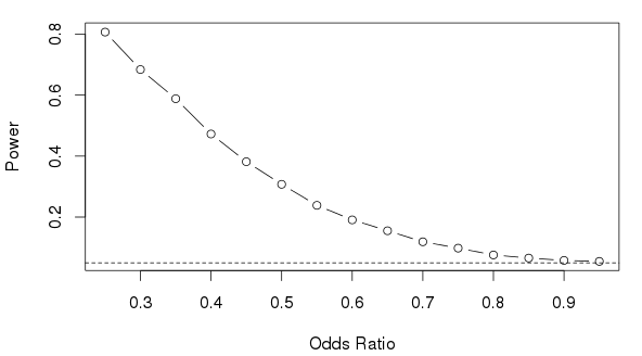
The code below demontrates the calculation of statistical power associated with sample of size 100 and odds ratio 0.25, where the control group frequencies of each category are as specified above. When executed, which takes some time, this gives about 80% power.

## power: n=50, OR=0.25
mean(replicate(10000, pocl_test(pocl_simulate(50, a=alph, b=c(0, log(0.25))))))

The figure below illustrates the power associated with a sequence of odds ratios. The dashed line represents the nominal type-I error rate 0.05.

Simulation-based power and precision analysis is a very powerful technique, which ensures that the reported statistical power reflects the intended statistical analysis (often times in research proposals, the proposed statistical analysis is not the same as that used to evaluate statistical power). In addition to the simple analysis described above, it is also possible to evaluate an adjusted analysis, i.e., the power to detect a treatment effect after adjustement for covariate effects. Of course, this requires that the latter effects be specified, and that there is some mechanism to simulate covariates. This can be a difficule task, but makes clear that there are many assumptions involved in a realistic power analysis.

Another advantage to simulation-based power analysis is that it requires implementation of the planned statistical procedure before the study begins, which ensures its feasibility and provides an opportunity to consider details that might otherwise be overlooked. Of course, it may also accelerate the 'real' analysis, once the data are collected.

Here is the complete R script:

## load MASS for polr()
library(MASS)
## specify frequencies of 11 ordered categories
prbs <- c(1,5,10,15,20,40,60,80,80,60,40)
prbs <- prbs/sum(prbs)
## sample 1000 observations with probabilities prbs
resp <- factor(replicate(1000, sample(0:10, 1, prob=prbs)),
               ordered=TRUE, levels=0:10)
## fit POCL model; extract intercepts (zeta here)
alph <- polr(resp~1)$zeta


## convenience functions
logit <- function(p) log(1/(1/p-1))
expit <- function(x) 1/(1/exp(x) + 1)

## block randomization
## n - number of randomizations
## m - block size
## levs - levels of treatment
block_rand <- function(n, m, levs=LETTERS[1:m]) {
  if(m %% length(levs) != 0)
    stop("length(levs) must be a factor of 'm'")
  k <- if(n%%m > 0) n%/%m + 1 else n%/%m
  l <- m %/% length(levs)
  factor(c(replicate(k, sample(rep(levs,l),
                               length(levs)*l, replace=FALSE))),levels=levs)
}

## simulate from POCL model
## n - sample size
## a - alpha
## b - beta
## levs - levels of outcome
pocl_simulate <- function(n, a, b, levs=0:length(a)) {
  dat <- data.frame(Treatment=block_rand(n,4,LETTERS[1:2])) 
  des <- model.matrix(~ 0 + Treatment, data=dat)
  nlev <- length(a) + 1
  yalp <- c(-Inf, a, Inf)
  xbet <- matrix(c(rep(0, nrow(des)),
                   rep(des %*% b , nlev-1),
                   rep(0, nrow(des))), nrow(des), nlev+1)
  prbs <- sapply(1:nlev, function(lev) {
    yunc <- rep(lev, nrow(des))
    expit(yalp[yunc+1] - xbet[cbind(1:nrow(des),yunc+1)]) - 
      expit(yalp[yunc]   - xbet[cbind(1:nrow(des),yunc)])
  })
  colnames(prbs) <- levs
  dat$y <- apply(prbs, 1, function(p) sample(levs, 1, prob=p))
  dat$y <- unname(factor(dat$y, levels=levs, ordered=TRUE))
  return(dat)
}

## Likelihood ratio test with 0.05 p-value threshold
## block randomization in blocks of size four to one
## of two treatment groups
## dat - data from pocl_simulate
pocl_test <- function(dat) {
  fit <- polr(y~Treatment, data=dat)
  anova(fit, update(fit, ~.-Treatment))$"Pr(Chi)"[2] < 0.05
}

## power: n=50, OR=0.25
mean(replicate(10000, pocl_test(pocl_simulate(50, a=alph, b=c(0, log(0.25))))))