
Problems In Estimating GARCH Parameters in R
Want to share your content on R-bloggers? click here if you have a blog, or here if you don't.
These days my research focuses on change point detection methods. These are statistical tests and procedures to detect a structural change in a sequence of data. An early example, from quality control, is detecting whether a machine became uncalibrated when producing a widget. There may be some measurement of interest, such as the diameter of a ball bearing, that we observe. The machine produces these widgets in sequence. Under the null hypothesis, the ball bearing’s mean diameter does not change, while under the alternative, at some unkown point in the manufacturing process the machine became uncalibrated and the mean diameter of the ball bearings changed. The test then decides between these two hypotheses.
These types of test matter to economists and financial sector workers as well, particularly for forecasting. Once again we have a sequence of data indexed by time; my preferred example is price of a stock, which people can instantly recognize as a time series given how common time series graphs for stocks are, but there are many more datasets such as a state’s GDP or the unemployment rate. Economists want to forecast these quantities using past data and statistics. One of the assumptions the statistical methods makes is that the series being forecasted is stationary: the data was generated by one process with a single mean, autocorrelation, distribution, etc. This assumption isn’t always tested yet it is critical to successful forecasting. Tests for structural change check this assumption, and if it turns out to be false, the forecaster may need to divide up their dataset when training their models.
I have written about these tests before, introducing the CUSUM statistic, one of the most popular statistics for detecting structural change. My advisor and a former Ph.D. student of his (currently a professor at the University of Waterloo, Greg Rice) developed a new test statistic that better detects structural changes that occur early or late in the dataset (imagine the machine producing widgets became uncalibrated just barely, and only the last dozen of the hundred widgets in the sample were affected). We’re in the process of making revisions requested by a journal to whom we submitted our paper, one of the revisions being a better example application (we initially worked with the wage/productivity data I discussed in the aforementioned blog post; the reviewers complained that these variables are codetermined so its nonsense to regress one on the other, a complaint I disagree with but I won’t plant my flag on to defend).
We were hoping to apply a version of our test to detecting structural change in GARCH models, a common model in financial time series. To my knowledge the “state of the art” R package for GARCH model estimation and inference (along with other work) is fGarch; in particular, the function garchFit() is used for estimating GARCH models from data. When we tried to use this function in our test, though, we were given obviously bad numbers (we had already done simulation studies to know what behavior to expect). The null hypothesis of no change was soundly rejected on simulated sequences where it was true. I never saw the test fail to reject the null hypothesis, even though the null hypothesis was always true. This was the case even for sample sizes of 10,000, hardly a small sample.
We thought the problem might lie with the estimation of the covariance matrix of the parameter estimates, and I painstakingly derived and programmed functions to get this matrix not using numerical differentiation procedures, yet this did not stop the bad behavior. Eventually my advisor and I last Wednesday played with garchFit() and decided that the function is to blame. The behavior of the function on simulated data is so erratic when estimating parameters (not necessarily the covariance matrix as we initially thought, though it’s likely polluted as well) the function is basically useless, to my knowledge.
This function should be well-known and it’s certainly possible that the problem lies with me, not fGarch (or perhaps there’s better packages out there). This strikes me as a function of such importance I should share my findings. In this article I show a series of numerical experiments demonstrating garchFit()‘s pathological behavior.
Basics on GARCH Models
The ")


People who follow finance1 noticed that returns to financial instruments (such as stocks or mutual funds) exhibit behavior known as volatility clustering. Some periods a financial instrument is relatively docile; there are not dramatic market movements. In others an instrument’s price can fluctuate greatly, and these periods are not one-off single-day movements but can last for a period of time. GARCH models were developed to model volatility clustering.
It is believed by some that even if a stock’s daily movement is essentially unforecastable (a stock is equally likely to over- or under-perform on any given day), the volatility is forecastable. Even for those who don’t have the hubris to believe anything about future returns can be forecasted these models are important. For example if one uses the model 


Estimating GARCH Parameters
The process I wrote down above is an infinite process; the index $latex $ can extend to negative numbers and beyond. Obviously in practice we don’t observe infinite sequences so if we want to work with


Below is the new sequence’s secret sauce:

We choose an initial value for this sequence (the theoretical
Naturally one of the most important tasks for these processes is estimating their parameters; for the 


")


")
 = f(x | \tilde{\sigma}_t^2)")
 = \frac{1}{\sqrt{2 \pi \tilde{\sigma}_t^2}} \exp\left(-\frac{x^2}{2 \tilde{\sigma}_t^2}\right)")
 = \prod_{t = 1}^T f(\epsilon_t | \tilde{\sigma}_t^2) = (2 \pi)^{-n/2} \prod_{t = 1}^T \tilde{\sigma}_t^{-1} \exp\left(-\frac{1}{2}\sum_{t = 1}^T \frac{\epsilon_t^2}{\tilde{\sigma}_t^2} \right)")
Like most likelihood methods, rather than optimize the quasi-likelihood function directly, statisticians try to optimize the log-likelihood, \right)")
 + \frac{\epsilon_t^2}{\tilde{\sigma}_t^2} \right)")
Note that 
It can be shown that the estimators for the parameters
Ideally, the parameters should behave like the process illustrated below.
library(ggplot2)

x <- rnorm(1000, sd = 1/3)
df <- t(sapply(50:1000, function(t) {
  return(c("mean" = mean(x[1:t]), "mean.se" = sd(x[1:t])/sqrt(t)))
}))
df <- as.data.frame(df)
df$t <- 50:1000
ggplot(df, aes(x = t, y = mean)) +
  geom_line() +
  geom_ribbon(aes(x = t, ymin = mean - 2 * mean.se, ymax = mean + 2 * mean.se),
              color = "grey", alpha = 0.5) +
  geom_hline(color = "blue", yintercept = 0) +
  coord_cartesian(ylim = c(-0.5, 0.5))

Behavior of Estimates by fGarch
Before continuing let’s generate a 
set.seed(110117)
library(fGarch)
x <- garchSim(garchSpec(model = list("alpha" = 0.2, "beta" = 0.2, "omega" = 0.2)),
              n.start = 1000, n = 1000)
plot(x)

Let’s see the parameters that the fGarch function garchFit() uses.
args(garchFit)


## function (formula = ~garch(1, 1), data = dem2gbp, init.rec = c("mci",
##     "uev"), delta = 2, skew = 1, shape = 4, cond.dist = c("norm",
##     "snorm", "ged", "sged", "std", "sstd", "snig", "QMLE"), include.mean = TRUE,
##     include.delta = NULL, include.skew = NULL, include.shape = NULL,
##     leverage = NULL, trace = TRUE, algorithm = c("nlminb", "lbfgsb",
##         "nlminb+nm", "lbfgsb+nm"), hessian = c("ropt", "rcd"),
##     control = list(), title = NULL, description = NULL, ...)
## NULL
The function provides a few options for distribution to maximize (cond.dist) and algorithm to use for optimization (algorithm). Here I will always choose cond.dist = QMLE, unless otherwise stated, to instruct the function to use QMLE estimators.
Here’s a single pass.
garchFit(data = x, cond.dist = "QMLE", include.mean = FALSE)


##
## Series Initialization:
##  ARMA Model:                arma
##  Formula Mean:              ~ arma(0, 0)
##  GARCH Model:               garch
##  Formula Variance:          ~ garch(1, 1)
##  ARMA Order:                0 0
##  Max ARMA Order:            0
##  GARCH Order:               1 1
##  Max GARCH Order:           1
##  Maximum Order:             1
##  Conditional Dist:          QMLE
##  h.start:                   2
##  llh.start:                 1
##  Length of Series:          1000
##  Recursion Init:            mci
##  Series Scale:              0.5320977
##
## Parameter Initialization:
##  Initial Parameters:          $params
##  Limits of Transformations:   $U, $V
##  Which Parameters are Fixed?  $includes
##  Parameter Matrix:
##                      U          V params includes
##     mu     -0.15640604   0.156406    0.0    FALSE
##     omega   0.00000100 100.000000    0.1     TRUE
##     alpha1  0.00000001   1.000000    0.1     TRUE
##     gamma1 -0.99999999   1.000000    0.1    FALSE
##     beta1   0.00000001   1.000000    0.8     TRUE
##     delta   0.00000000   2.000000    2.0    FALSE
##     skew    0.10000000  10.000000    1.0    FALSE
##     shape   1.00000000  10.000000    4.0    FALSE
##  Index List of Parameters to be Optimized:
##  omega alpha1  beta1
##      2      3      5
##  Persistence:                  0.9
##
##
## --- START OF TRACE ---
## Selected Algorithm: nlminb
##
## R coded nlminb Solver:
##
##   0:     1419.0152: 0.100000 0.100000 0.800000
##   1:     1418.6616: 0.108486 0.0998447 0.804683
##   2:     1417.7139: 0.109746 0.0909961 0.800931
##   3:     1416.7807: 0.124977 0.0795152 0.804400
##   4:     1416.7215: 0.141355 0.0446605 0.799891
##   5:     1415.5139: 0.158059 0.0527601 0.794304
##   6:     1415.2330: 0.166344 0.0561552 0.777108
##   7:     1415.0415: 0.195230 0.0637737 0.743465
##   8:     1415.0031: 0.200862 0.0576220 0.740088
##   9:     1414.9585: 0.205990 0.0671331 0.724721
##  10:     1414.9298: 0.219985 0.0713468 0.712919
##  11:     1414.8226: 0.230628 0.0728325 0.697511
##  12:     1414.4689: 0.325750 0.0940514 0.583114
##  13:     1413.4560: 0.581449 0.143094 0.281070
##  14:     1413.2804: 0.659173 0.157127 0.189282
##  15:     1413.2136: 0.697840 0.155964 0.150319
##  16:     1413.1467: 0.720870 0.142550 0.137645
##  17:     1413.1416: 0.726527 0.138146 0.135966
##  18:     1413.1407: 0.728384 0.137960 0.134768
##  19:     1413.1392: 0.731725 0.138321 0.132991
##  20:     1413.1392: 0.731146 0.138558 0.133590
##  21:     1413.1392: 0.730849 0.138621 0.133850
##  22:     1413.1392: 0.730826 0.138622 0.133869
##
## Final Estimate of the Negative LLH:
##  LLH:  782.211    norm LLH:  0.782211
##     omega    alpha1     beta1
## 0.2069173 0.1386221 0.1338686
##
## R-optimhess Difference Approximated Hessian Matrix:
##            omega     alpha1      beta1
## omega  -8858.897 -1839.6144 -2491.9827
## alpha1 -1839.614  -782.8005  -531.7393
## beta1  -2491.983  -531.7393  -729.7246
## attr(,"time")
## Time difference of 0.04132652 secs
##
## --- END OF TRACE ---
##
##
## Time to Estimate Parameters:
##  Time difference of 0.3866439 secs


##
## Title:
##  GARCH Modelling
##
## Call:
##  garchFit(data = x, cond.dist = "QMLE", include.mean = FALSE)
##
## Mean and Variance Equation:
##  data ~ garch(1, 1)
## <environment: 0xa636ba4>
##  [data = x]
##
## Conditional Distribution:
##  QMLE
##
## Coefficient(s):
##   omega   alpha1    beta1
## 0.20692  0.13862  0.13387
##
## Std. Errors:
##  robust
##
## Error Analysis:
##         Estimate  Std. Error  t value Pr(>|t|)
## omega    0.20692     0.05102    4.056    5e-05 ***
## alpha1   0.13862     0.04928    2.813  0.00491 **
## beta1    0.13387     0.18170    0.737  0.46128
## ---
## Signif. codes:  0 '***' 0.001 '**' 0.01 '*' 0.05 '.' 0.1 ' ' 1
##
## Log Likelihood:
##  -782.211    normalized:  -0.782211
##
## Description:
##  Thu Nov  2 13:01:14 2017 by user:
The parameters are not necessarily near the true parameters. One might initially attribute this to just randomness, but that doesn’t seem to be the case.
For example, what fit do I get when I fit the model on the first 500 data points?
garchFit(data = x[1:500], cond.dist = "QMLE", include.mean = FALSE)


##
## Series Initialization:
##  ARMA Model:                arma
##  Formula Mean:              ~ arma(0, 0)
##  GARCH Model:               garch
##  Formula Variance:          ~ garch(1, 1)
##  ARMA Order:                0 0
##  Max ARMA Order:            0
##  GARCH Order:               1 1
##  Max GARCH Order:           1
##  Maximum Order:             1
##  Conditional Dist:          QMLE
##  h.start:                   2
##  llh.start:                 1
##  Length of Series:          500
##  Recursion Init:            mci
##  Series Scale:              0.5498649
##
## Parameter Initialization:
##  Initial Parameters:          $params
##  Limits of Transformations:   $U, $V
##  Which Parameters are Fixed?  $includes
##  Parameter Matrix:
##                      U           V params includes
##     mu     -0.33278068   0.3327807    0.0    FALSE
##     omega   0.00000100 100.0000000    0.1     TRUE
##     alpha1  0.00000001   1.0000000    0.1     TRUE
##     gamma1 -0.99999999   1.0000000    0.1    FALSE
##     beta1   0.00000001   1.0000000    0.8     TRUE
##     delta   0.00000000   2.0000000    2.0    FALSE
##     skew    0.10000000  10.0000000    1.0    FALSE
##     shape   1.00000000  10.0000000    4.0    FALSE
##  Index List of Parameters to be Optimized:
##  omega alpha1  beta1
##      2      3      5
##  Persistence:                  0.9
##
##
## --- START OF TRACE ---
## Selected Algorithm: nlminb
##
## R coded nlminb Solver:
##
##   0:     706.37230: 0.100000 0.100000 0.800000
##   1:     706.27437: 0.103977 0.100309 0.801115
##   2:     706.19091: 0.104824 0.0972295 0.798477
##   3:     706.03116: 0.112782 0.0950253 0.797812
##   4:     705.77389: 0.122615 0.0858136 0.788169
##   5:     705.57316: 0.134608 0.0913105 0.778144
##   6:     705.43424: 0.140011 0.0967118 0.763442
##   7:     705.19541: 0.162471 0.102711 0.739827
##   8:     705.16325: 0.166236 0.0931680 0.737563
##   9:     705.09943: 0.168962 0.100977 0.731085
##  10:     704.94924: 0.203874 0.0958205 0.702986
##  11:     704.78210: 0.223975 0.108606 0.664678
##  12:     704.67414: 0.250189 0.122959 0.630886
##  13:     704.60673: 0.276532 0.131788 0.595346
##  14:     704.52185: 0.335952 0.146435 0.520961
##  15:     704.47725: 0.396737 0.157920 0.448557
##  16:     704.46540: 0.442499 0.164111 0.396543
##  17:     704.46319: 0.440935 0.161566 0.400606
##  18:     704.46231: 0.442951 0.159225 0.400940
##  19:     704.46231: 0.443022 0.159284 0.400863
##  20:     704.46230: 0.443072 0.159363 0.400851
##  21:     704.46230: 0.443112 0.159367 0.400807
##
## Final Estimate of the Negative LLH:
##  LLH:  405.421    norm LLH:  0.810842
##     omega    alpha1     beta1
## 0.1339755 0.1593669 0.4008074
##
## R-optimhess Difference Approximated Hessian Matrix:
##            omega     alpha1      beta1
## omega  -8491.005 -1863.4127 -2488.5700
## alpha1 -1863.413  -685.6071  -585.4327
## beta1  -2488.570  -585.4327  -744.1593
## attr(,"time")
## Time difference of 0.02322888 secs
##
## --- END OF TRACE ---
##
##
## Time to Estimate Parameters:
##  Time difference of 0.1387401 secs


##
## Title:
##  GARCH Modelling
##
## Call:
##  garchFit(data = x[1:500], cond.dist = "QMLE", include.mean = FALSE)
##
## Mean and Variance Equation:
##  data ~ garch(1, 1)
## <environment: 0xa85f084>
##  [data = x[1:500]]
##
## Conditional Distribution:
##  QMLE
##
## Coefficient(s):
##   omega   alpha1    beta1
## 0.13398  0.15937  0.40081
##
## Std. Errors:
##  robust
##
## Error Analysis:
##         Estimate  Std. Error  t value Pr(>|t|)
## omega    0.13398     0.11795    1.136   0.2560
## alpha1   0.15937     0.07849    2.030   0.0423 *
## beta1    0.40081     0.44228    0.906   0.3648
## ---
## Signif. codes:  0 '***' 0.001 '**' 0.01 '*' 0.05 '.' 0.1 ' ' 1
##
## Log Likelihood:
##  -405.421    normalized:  -0.810842
##
## Description:
##  Thu Nov  2 13:01:15 2017 by user:
Notice that the parameter beta1) changed dramatically. How about a different cutoff?
garchFit(data = x[1:200], cond.dist = "QMLE", include.mean = FALSE)


##
## Series Initialization:
##  ARMA Model:                arma
##  Formula Mean:              ~ arma(0, 0)
##  GARCH Model:               garch
##  Formula Variance:          ~ garch(1, 1)
##  ARMA Order:                0 0
##  Max ARMA Order:            0
##  GARCH Order:               1 1
##  Max GARCH Order:           1
##  Maximum Order:             1
##  Conditional Dist:          QMLE
##  h.start:                   2
##  llh.start:                 1
##  Length of Series:          200
##  Recursion Init:            mci
##  Series Scale:              0.5746839
##
## Parameter Initialization:
##  Initial Parameters:          $params
##  Limits of Transformations:   $U, $V
##  Which Parameters are Fixed?  $includes
##  Parameter Matrix:
##                      U           V params includes
##     mu     -0.61993813   0.6199381    0.0    FALSE
##     omega   0.00000100 100.0000000    0.1     TRUE
##     alpha1  0.00000001   1.0000000    0.1     TRUE
##     gamma1 -0.99999999   1.0000000    0.1    FALSE
##     beta1   0.00000001   1.0000000    0.8     TRUE
##     delta   0.00000000   2.0000000    2.0    FALSE
##     skew    0.10000000  10.0000000    1.0    FALSE
##     shape   1.00000000  10.0000000    4.0    FALSE
##  Index List of Parameters to be Optimized:
##  omega alpha1  beta1
##      2      3      5
##  Persistence:                  0.9
##
##
## --- START OF TRACE ---
## Selected Algorithm: nlminb
##
## R coded nlminb Solver:
##
##   0:     280.63354: 0.100000 0.100000 0.800000
##   1:     280.63302: 0.100315 0.100088 0.800223
##   2:     280.63262: 0.100695 0.0992822 0.800059
##   3:     280.63258: 0.102205 0.0983397 0.800404
##   4:     280.63213: 0.102411 0.0978709 0.799656
##   5:     280.63200: 0.102368 0.0986702 0.799230
##   6:     280.63200: 0.101930 0.0984977 0.800005
##   7:     280.63200: 0.101795 0.0983937 0.799987
##   8:     280.63197: 0.101876 0.0984197 0.799999
##   9:     280.63197: 0.102003 0.0983101 0.799965
##  10:     280.63197: 0.102069 0.0983780 0.799823
##  11:     280.63197: 0.102097 0.0983703 0.799827
##  12:     280.63197: 0.102073 0.0983592 0.799850
##  13:     280.63197: 0.102075 0.0983616 0.799846
##
## Final Estimate of the Negative LLH:
##  LLH:  169.8449    norm LLH:  0.8492246
##      omega     alpha1      beta1
## 0.03371154 0.09836156 0.79984610
##
## R-optimhess Difference Approximated Hessian Matrix:
##             omega    alpha1     beta1
## omega  -26914.901 -6696.498 -8183.925
## alpha1  -6696.498 -2239.695 -2271.547
## beta1   -8183.925 -2271.547 -2733.098
## attr(,"time")
## Time difference of 0.02161336 secs
##
## --- END OF TRACE ---
##
##
## Time to Estimate Parameters:
##  Time difference of 0.09229803 secs


##
## Title:
##  GARCH Modelling
##
## Call:
##  garchFit(data = x[1:200], cond.dist = "QMLE", include.mean = FALSE)
##
## Mean and Variance Equation:
##  data ~ garch(1, 1)
## <environment: 0xad38a84>
##  [data = x[1:200]]
##
## Conditional Distribution:
##  QMLE
##
## Coefficient(s):
##    omega    alpha1     beta1
## 0.033712  0.098362  0.799846
##
## Std. Errors:
##  robust
##
## Error Analysis:
##         Estimate  Std. Error  t value Pr(>|t|)
## omega    0.03371     0.01470    2.293   0.0218 *
## alpha1   0.09836     0.04560    2.157   0.0310 *
## beta1    0.79985     0.03470   23.052   <2e-16 ***
## ---
## Signif. codes:  0 '***' 0.001 '**' 0.01 '*' 0.05 '.' 0.1 ' ' 1
##
## Log Likelihood:
##  -169.8449    normalized:  -0.8492246
##
## Description:
##  Thu Nov  2 13:01:15 2017 by user:
For 200 observations
Let’s dive deeper into this. I’ve conducted a number of numerical experiments on the University of Utah Mathematics department’s supercomputer. Below is a helper function to extract the coefficients and standard errors for a particular fit by garchFit() (suppressing all of garchFit()‘s output in the process).
getFitData <- function(x, cond.dist = "QMLE", include.mean = FALSE, ...) {
  args <- list(...)
  args$data = x
  args$cond.dist = cond.dist
  args$include.mean = include.mean

  log <- capture.output({
    fit <- do.call(garchFit, args = args)
  })

  res <- coef(fit)
  res[paste0(names(fit@fit$se.coef), ".se")] <- fit@fit$se.coef
  return(res)
}
The first experiment is to compute the coefficients of this particular series at each possible end point.
(The following code block is not evaluated when this document is knitted; I have saved the results in a Rda file. This will be the case for every code block that involves parallel computation. I performed these computations on the University of Utah mathematics department’s supercomputer, saving the results for here.)
library(doParallel)

set.seed(110117)

cl <- makeCluster(detectCores() - 1)
registerDoParallel(cl)

x <- garchSim(garchSpec(model = list(alpha = 0.2, beta = 0.2, omega = 0.2)),
              n.start = 1000, n = 1000)

params <- foreach(t = 50:1000, .combine = rbind,
                  .packages = c("fGarch")) %dopar% {
                    getFitData(x[1:t])
}
rownames(params) <- 50:1000
Below I plot these coefficients, along with a region corresponding to double the standard error. This region should roughly correspond to 95% confidence intervals.
params_df <- as.data.frame(params)
params_df$t <- as.numeric(rownames(params))
ggplot(params_df) +
  geom_line(aes(x = t, y = beta1)) +
  geom_hline(yintercept = 0.2, color = "blue") +
  geom_ribbon(aes(x = t, ymin = beta1 - 2 * beta1.se,
                  ymax = beta1 + 2 * beta1.se),
              color = "grey", alpha = 0.5) +
  ylab(expression(hat(beta))) +
  scale_y_continuous(breaks = c(0, 0.2, 0.25, 0.5, 1)) +
  coord_cartesian(ylim = c(0, 1))
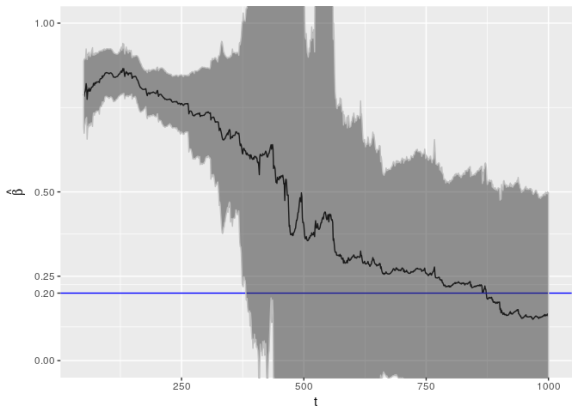
This is an alarming picture (but not the most alarming I’ve seen; this is one of the better cases). Notice that the confidence interval fails to capture the true value of 
Let’s see how the other parameters behave.
library(reshape2)
library(plyr)
library(dplyr)

param_reshape <- function(p) {
  p <- as.data.frame(p)
  p$t <- as.integer(rownames(p))

  pnew <- melt(p, id.vars = "t", variable.name = "parameter")

  pnew$parameter <- as.character(pnew$parameter)
  pnew.se <- pnew[grepl("*.se", pnew$parameter), ]
  pnew.se$parameter <- sub(".se", "", pnew.se$parameter)
  names(pnew.se)[3] <- "se"
  pnew <- pnew[!grepl("*.se", pnew$parameter), ]

  return(join(pnew, pnew.se, by = c("t", "parameter"), type = "inner"))
}


ggp <- ggplot(param_reshape(params), aes(x = t, y = value)) +
  geom_line() + geom_ribbon(aes(ymin = value - 2 * se,
                                ymax = value + 2 * se), color = "grey",
                            alpha = 0.5) +
  geom_hline(yintercept = 0.2, color = "blue") +
  scale_y_continuous(breaks = c(0, 0.2, 0.25, 0.5, 0.75, 1)) +
  coord_cartesian(ylim = c(0, 1)) +
  facet_grid(. ~ parameter)

print(ggp + ggtitle("NLMINB Optimization"))

The phenomenon is not limited to
This behavior isn’t unusual; it’s typical. Below are plots for similar series generated with different seeds.
seeds <- c(103117, 123456, 987654, 101010, 8675309, 81891, 222222, 999999,
           110011)

experiments1 <- foreach(s = seeds) %do% {
  set.seed(s)
  x <- garchSim(garchSpec(model = list(alpha = 0.2, beta = 0.2, omega = 0.2)),
                n.start = 1000, n = 1000)
  params <- foreach(t = 50:1000, .combine = rbind,
                    .packages = c("fGarch")) %dopar% {
                      getFitData(x[1:t])
  }
  rownames(params) <- 50:1000
  params
}
names(experiments1) <- seeds


experiments1 <- lapply(experiments1, param_reshape)
names(experiments1) <- c(103117, 123456, 987654, 101010, 8675309, 81891,
                         222222, 999999, 110011)
experiments1_df <- ldply(experiments1, .id = "seed")
head(experiments1_df)


##     seed  t parameter     value        se
## 1 103117 50     omega 0.1043139 0.9830089
## 2 103117 51     omega 0.1037479 4.8441246
## 3 103117 52     omega 0.1032197 4.6421147
## 4 103117 53     omega 0.1026722 1.3041128
## 5 103117 54     omega 0.1020266 0.5334988
## 6 103117 55     omega 0.2725939 0.6089607


ggplot(experiments1_df, aes(x = t, y = value)) +
  geom_line() + geom_ribbon(aes(ymin = value - 2 * se, ymax = value + 2 * se),
                            color = "grey", alpha = 0.5) +
  geom_hline(yintercept = 0.2, color = "blue") +
  scale_y_continuous(breaks = c(0, 0.2, 0.25, 0.5, 0.75, 1)) +
  coord_cartesian(ylim = c(0, 1)) +
  facet_grid(seed ~ parameter) +
  ggtitle("Successive parameter estimates using NLMINB optimization")

In this plot we see pathologies of other kinds for
The other parameters are not without their own pathologies but the situation does not seem quite so grim. It’s possible the pathologies we do see are tied to estimation of 
set.seed(110117)

x <- garchSim(garchSpec(model = list(alpha = 0.2, beta = 0.2, omega = 0.2)),
              n.start = 1000, n = 1000)

xarch <- garchSim(garchSpec(model = list(omega = 0.2, alpha = 0.2, beta = 0)),
                  n.start = 1000, n = 1000)
params_arch <- foreach(t = 50:1000, .combine = rbind,
                       .packages = c("fGarch")) %dopar% {
                         getFitData(xarch[1:t], formula = ~ garch(1, 0))
}
rownames(params_arch) <- 50:1000


print(ggp %+% param_reshape(params_arch) + ggtitle("ARCH(1) Model"))

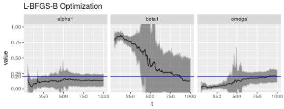
The pathology appears to be numerical in nature and closely tied to garchFit(), by default, uses nlminb() (a quasi-Newton method with constraints) for solving the optimization problem, using a numerically-computed gradient. We can choose alternative methods, though; we can use the L-BFGS-B method, and we can spice both with the Nelder-Mead method.
Unfortunately these alternative optimization algorithms don’t do better; they may even do worse.
# lbfgsb algorithm
params_lbfgsb <- foreach(t = 50:1000, .combine = rbind,
                         .packages = c("fGarch")) %dopar% {
                           getFitData(x[1:t], algorithm = "lbfgsb")
}
rownames(params_lbfgsb) <- 50:1000

# nlminb+nm algorithm
params_nlminbnm <- foreach(t = 50:1000, .combine = rbind,
                           .packages = c("fGarch")) %dopar% {
                             getFitData(x[1:t], algorithm = "nlminb+nm")
}
rownames(params_nlminbnm) <- 50:1000

# lbfgsb+nm algorithm
params_lbfgsbnm <- foreach(t = 50:1000, .combine = rbind,
                           .packages = c("fGarch")) %dopar% {
                             getFitData(x[1:t], algorithm = "lbfgsb+nm")
}
rownames(params_lbfgsbnm) <- 50:1000

# cond.dist is norm (default)
params_norm <- foreach(t = 50:1000, .combine = rbind,
                       .packages = c("fGarch")) %dopar% {
                         getFitData(x[1:t], cond.dist = "norm")
}
rownames(params_norm) <- 50:1000


print(ggp %+% param_reshape(params_lbfgsb) + ggtitle("L-BFGS-B Optimization"))
print(ggp %+% param_reshape(params_nlminbnm) +
        ggtitle("nlminb Optimization with Nelder-Mead"))

print(ggp %+% param_reshape(params_lbfgsbnm) +
        ggtitle("L-BFGS-B Optimization with Nelder-Mead"))

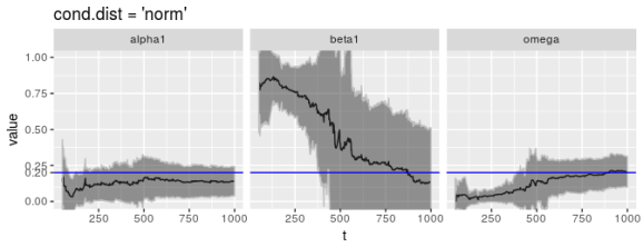
Admittedly, though, QMLE is not the default estimation method garchFit() uses. The default is the Normal distribution. Unfortunately this is no better.
print(ggp %+% param_reshape(params_norm) +
        ggtitle("cond.dist = 'norm'"))
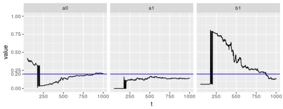
On CRAN, fGarch has not seen an update since 2013! It’s possible that fGarch is starting to show its age and newer packages have addressed some of the problems I’ve highlighted here. The package tseries provides a function garch() that also fits
Unfortunately, garch() doesn’t do much better; in fact, it appears to be much worse. Once again, the problem lies with
library(tseries)

getFitDatagarch <- function(x) {
  garch(x)$coef
}

params_tseries <- foreach(t = 50:1000, .combine = rbind,
                          .packages = c("tseries")) %dopar% {
                            getFitDatagarch(x[1:t])
}
rownames(params_tseries) <- 50:1000


param_reshape_tseries <- function(p) {
  p <- as.data.frame(p)
  p$t <- as.integer(rownames(p))

  pnew <- melt(p, id.vars = "t", variable.name = "parameter")

  pnew$parameter <- as.character(pnew$parameter)

  return(pnew)
}

ggplot(param_reshape_tseries(params_tseries), aes(x = t, y = value)) +
  geom_line() + geom_hline(yintercept = 0.2, color = "blue") +
  scale_y_continuous(breaks = c(0, 0.2, 0.25, 0.5, 0.75, 1)) +
  coord_cartesian(ylim = c(0, 1)) +
  facet_grid(. ~ parameter)
All of these experiments were performed on fixed (yet randomly chosen) sequences. They suggest that especially for sample sizes of less than, say, 300 (possibly larger) distributional guarantees for the estimates of
I simulated 10,000
experiments2 <- foreach(n = c(100, 500, 1000)) %do% {
  mat <- foreach(i = 1:10000, .combine = rbind,
                 .packages = c("fGarch")) %dopar% {
    x <- garchSim(garchSpec(model = list(omega = 0.2, alpha = 0.2,
                                         beta = 0.2)), n.start = 1000,
                  n = n)
    getFitData(x)
  }
  rownames(mat) <- NULL
  mat
}
names(experiments2) <- c(100, 500, 1000)

save(params, x, experiments1, xarch, params_arch, params_lbfgsb,
     params_nlminbnm, params_lbfgsbnm, params_norm, params_tseries,
     experiments2, file="garchfitexperiments.Rda")


param_sim <- lapply(experiments2, function(mat) {
  df <- as.data.frame(mat)
  df <- df[c("omega", "alpha1", "beta1")]
  return(df)
}) %>% ldply(.id = "n")
param_sim <- param_sim %>% melt(id.vars = "n", variable.name = "parameter")
head(param_sim)


##     n parameter        value
## 1 100     omega 8.015968e-02
## 2 100     omega 2.493595e-01
## 3 100     omega 2.300699e-01
## 4 100     omega 3.674244e-07
## 5 100     omega 2.697577e-03
## 6 100     omega 2.071737e-01


ggplot(param_sim, aes(x = value)) + geom_density(fill = "grey", alpha = 0.7) +
  geom_vline(xintercept = 0.2, color = "blue") +
  facet_grid(n ~ parameter)

When the sample size is 100, these estimators are far from reliable. garchFit() do not capture this behavior. For larger sample sizes
What bothers me most is that a sample size of 1,000 strikes me as being a large sample size. If one were looking at daily data for, say, stock prices, this sample size roughly corresponds to maybe 4 years of data. This suggests to me that this pathological behavior is affecting GARCH models people are trying to estimate now and use in models.
Conclusion
An article by John C. Nash entitled “On best practice optimization methods in R”, published in the Journal of Statistical Software in September 2014, discussed the need for better optimization practices in R. In particular, he highlighted, among others, the methods garchFit() uses (or at least their R implementation) as outdated. He argues for greater awareness in the community for optimization issues and for greater flexibility in packages, going beyond merely using different algorithms provided by optim().
The issues I highlighted in this article made me more aware of the importance of choice in optimization methods. My initial objective was to write a function for performing statistical tests depending structural change in GARCH models. These tests rely heavily on successive estimation of the parameters of models as I demonstrated here. At minimum my experiments show that the variation in the parameters isn’t being captured adequately by standard errors, but also there’s a potential for unacceptably high instability in parameter estimates. They’re so unstable it would take a miracle for the test to not reject the null hypothesis of no change. After all, just looking at the pictures of simulated data and one might conclude that the alternative hypothesis of structural change is true. Thus every time I have tried to implement our test on data where the null hypothesis was supposedly true, the test unequivocally rejected it with $p$-values of essentially 0.
I have heard people conducting hypothesis testing for detecting structural change in GARCH models so I would not be surprised if the numerical instability I have written about here can be avoided. This is a subject I admittedly know little about and I hope that if someone in the R community has already observed this behavior and knows how to resolve it they let me know in the comments or via e-mail. I may write a retraction and show how to produce stable estimates of the parameters with garchFit(). Perhaps the key lies in the function garchFitControl().
I’ve also thought about writing my own optimization routine tailored to my test. Prof. Nash emphasized in his paper the importance of tailoring optimization routines to the needs of particular problems. I’ve written down the quantity to optimize and I have a formula for the gradient and Hessian matrix of the
Already though this makes the problem more difficult than I initially thought finding an example for our test would be. I’m planning on tabling detecting structural change in GARCH models for now and using instead an example involving merely linear regression (a much more tractable problem). But I hope to hear others’ input on what I’ve written here.
sessionInfo()


## R version 3.3.3 (2017-03-06)
## Platform: i686-pc-linux-gnu (32-bit)
## Running under: Ubuntu 16.04.2 LTS
##
## locale:
##  [1] LC_CTYPE=en_US.UTF-8       LC_NUMERIC=C
##  [3] LC_TIME=en_US.UTF-8        LC_COLLATE=en_US.UTF-8
##  [5] LC_MONETARY=en_US.UTF-8    LC_MESSAGES=en_US.UTF-8
##  [7] LC_PAPER=en_US.UTF-8       LC_NAME=C
##  [9] LC_ADDRESS=C               LC_TELEPHONE=C
## [11] LC_MEASUREMENT=en_US.UTF-8 LC_IDENTIFICATION=C
##
## attached base packages:
## [1] stats     graphics  grDevices utils     datasets  methods   base
##
## other attached packages:
## [1] dplyr_0.7.2           plyr_1.8.4            reshape2_1.4.2
## [4] fGarch_3010.82.1      fBasics_3011.87       timeSeries_3022.101.2
## [7] timeDate_3012.100     ggplot2_2.2.1
##
## loaded via a namespace (and not attached):
##  [1] Rcpp_0.12.11     bindr_0.1        knitr_1.17       magrittr_1.5
##  [5] munsell_0.4.3    colorspace_1.3-2 R6_2.2.0         rlang_0.1.2
##  [9] stringr_1.2.0    tools_3.3.3      grid_3.3.3       gtable_0.2.0
## [13] htmltools_0.3.6  assertthat_0.1   yaml_2.1.14      lazyeval_0.2.0
## [17] rprojroot_1.2    digest_0.6.12    tibble_1.3.4     bindrcpp_0.2
## [21] glue_1.1.1       evaluate_0.10    rmarkdown_1.6    labeling_0.3
## [25] stringi_1.1.5    scales_0.4.1     backports_1.0.5  pkgconfig_2.0.1
- Bollerslev introduced GARCH models in his 1986 paper entitled “General autoregressive conditional heteroscedasticity”. ↩
- See the book GARCH Models: Structure, Statistical Inference and Financial Applications, by Christian Francq and Jean-Michel Zakoian. ↩

R-bloggers.com offers daily e-mail updates about R news and tutorials about learning R and many other topics. Click here if you're looking to post or find an R/data-science job.
Want to share your content on R-bloggers? click here if you have a blog, or here if you don't.