Obtaining the number of components from cross validation of principal components regression
Want to share your content on R-bloggers? click here if you have a blog, or here if you don't.
Principal components (PC) regression is a common dimensionality reduction technique in supervised learning. The R lab for PC regression in James et al.’s Introduction to Statistical Learning is a popular intro for how to perform PC regression in R: it is on p256-257 of the book (p270-271 of the PDF).
As in the lab, the code below runs PC regression on the Hitters data to predict Salary:
library(ISLR)
data(Hitters)
library(pls)
set.seed(2)
pcr.fit = pcr(Salary ~ ., data = Hitters, scale = TRUE,
    validation = "CV")
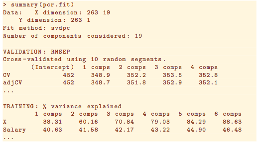
The result of the fit can be seen by calling summary(pcr.fit):

Taken from ISLR Section 6.7.1.
When predicting the response on test data, we would choose the number of components based on which model gave the smallest cross validation (CV) error. What is strange in this lab is that they do not pull out the “optimal” number of components via code! Instead, they make a plot of CV error, visually identified the number of components giving smallest CV error (7 in this case), then predicted on the test set with 7 hardcoded. Here is their code:
# get indices for training set
set.seed(1)
train = sample(1:nrow(Hitters), nrow(Hitters) / 2)

# perform PC regression with CV on just the training set
set.seed(1)
pcr.fit = pcr(Salary ~ ., data = Hitters, subset = train,
              scale = TRUE, validation = "CV")

# plot of CV error
validationplot(pcr.fit, val.type = "MSEP")
# visual inspection of plot: 7 gives min CV error!

# predict on test data
pcr.pred = predict(pcr.fit, x[-train,], ncomp = 7)
This method of identifying the number of components with smallest CV error is not ideal. Here is the output of validationplot:

I think it’s actually quite hard to tell by eye that 7 principal components is the best choice! In any case, we might want a programmatic way of finding the best number of components (according to CV) so that we don’t have to stop our data modeling pipeline to make a visual check.
It turns out that we can use the RMSEP function to pull out the CV and adjCV table that we saw in summary(pcr.fit):
RMSEP(pcr.fit)
#        (Intercept)  1 comps  2 comps  3 comps  4 comps  5 comps  6 comps  7 comps  8 comps  9 comps  10 comps
# CV             488    386.2    387.3    387.0    387.9    390.9    383.8    382.5    388.0    388.1     385.2
# adjCV          488    385.1    386.2    385.7    386.5    389.5    381.1    380.5    385.7    385.7     382.7
#        11 comps  12 comps  13 comps  14 comps  15 comps  16 comps  17 comps  18 comps  19 comps
# CV        385.9     387.1     392.7     408.1     395.3     386.6     394.0     399.6     405.6
# adjCV     383.3     384.5     390.1     404.6     391.3     382.8     389.8     394.8     400.5
To get at the individual values in the table, we need to access val key and subset appropriately:
cverr <- RMSEP(pcr.fit)$val[1,,]
imin <- which.min(cverr) - 1
Note that we have to subtract 1, since the model with no principal components is included in the output of RMSEP(pcr.fit) as well. If we wish to get the best number of PCs based on adjusted CV instead, we could amend that first line of code to RMSEP(pcr.fit)$val[1,,].
R-bloggers.com offers daily e-mail updates about R news and tutorials about learning R and many other topics. Click here if you're looking to post or find an R/data-science job.
Want to share your content on R-bloggers? click here if you have a blog, or here if you don't.
