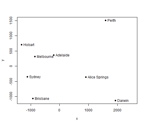
This page shows Multidimensional Scaling (MDS) with R. It demonstrates with an example of automatic layout of Australian cities based on distances between them. The layout obtained with MDS is very close to their locations on a map.

At first, the data of distances between 8 city in Australia are loaded from http://rosetta.reltech.org/TC/v15/Mapping/data/dist-Aus.csv.

dist.au <- read.csv("http://rosetta.reltech.org/TC/v15/Mapping/data/dist-Aus.csv")

Alternatively, we can download the file first and then read it into R from local drive.

dist.au <- read.csv("dist-Aus.csv")
dist.au

##    X    A   AS    B    D    H    M    P    S
## 1  A    0 1328 1600 2616 1161  653 2130 1161
## 2 AS 1328    0 1962 1289 2463 1889 1991 2026
## 3  B 1600 1962    0 2846 1788 1374 3604  732
## 4  D 2616 1289 2846    0 3734 3146 2652 3146
## 5  H 1161 2463 1788 3734    0  598 3008 1057
## 6  M  653 1889 1374 3146  598    0 2720  713
## 7  P 2130 1991 3604 2652 3008 2720    0 3288
## 8  S 1161 2026  732 3146 1057  713 3288    0

Then we remove the frist column, acronyms of cities, and set them to row names.

row.names(dist.au) <- dist.au[, 1]
dist.au <- dist.au[, -1]
dist.au

##       A   AS    B    D    H    M    P    S
## A     0 1328 1600 2616 1161  653 2130 1161
## AS 1328    0 1962 1289 2463 1889 1991 2026
## B  1600 1962    0 2846 1788 1374 3604  732
## D  2616 1289 2846    0 3734 3146 2652 3146
## H  1161 2463 1788 3734    0  598 3008 1057
## M   653 1889 1374 3146  598    0 2720  713
## P  2130 1991 3604 2652 3008 2720    0 3288
## S  1161 2026  732 3146 1057  713 3288    0

After that, we run Multidimensional Scaling (MDS) with function cmdscale(), and get x and y coordinates.

fit <- cmdscale(dist.au, eig = TRUE, k = 2)
x <- fit$points[, 1]
y <- fit$points[, 2]

Then we visualise the result, which shows the positions of cities are very close to their relative locations on a map.

plot(x, y, pch = 19, xlim = range(x) + c(0, 600))
city.names <- c("Adelaide", "Alice Springs", "Brisbane", "Darwin", "Hobart", 
    "Melbourne", "Perth", "Sydney")
text(x, y, pos = 4, labels = city.names)

By flipping both x- and y-axis, Darwin and Brisbane are moved to the top (north), which makes it easier to compare with a map.

x <- 0 - x
y <- 0 - y
plot(x, y, pch = 19, xlim = range(x) + c(0, 600))
text(x, y, pos = 4, labels = city.names)

MDS is also implemented in the igraph package as layout.mds.

library(igraph)
g <- graph.full(nrow(dist.au))
V(g)$label <- city.names
layout <- layout.mds(g, dist = as.matrix(dist.au))
plot(g, layout = layout, vertex.size = 3)