Dataset here.

We are going to perform a linear mixed effects analysis of the relationship between height and treatment of trees, as studied over a period of time.

Begin by reading in the data and making sure that the variables have the appropriate datatype.

tree<- read.csv(path, header=T,sep=",")
tree$ID<- factor(tree$ID)
tree$plotnr <- factor(tree$plotnr)

Plot the initial graph to get a sense of the relationship between the variables.

library(lattice)
bwplot(height ~ Date|treat,data=tree)

There seems to be a linear-ish relationship between height and time . The height increases over time.The effect of the treatments(I,IL,C,F) is not clear at this point.

Based on the linear nature of relationship, we can model time to be numeric, i.e. , number of days.

tree$Date<- as.Date(tree$Date)
tree$time<- as.numeric(tree$Date - min(tree$Date))

The data shows us that the data was collected from the same plot on multiple dates, making it  a candidate for repeated measures.

Let’s visually check for the by-plot variability.

boxplot(height ~ plotnr,data=tree)

The variation between plots isn’t big – but there are still noticeable differences which will need to be accounted for in our model.

Let’s fit two models : one with interaction between the predictors and one without.

library(lme4)
library(lmerTest)

#fit a model

mod <- lmer(height ~ time + treat + (1|plotnr),data=tree) #without interaction
mod.int <- lmer(height ~ time * treat + (1|plotnr),data=tree) #with interaction

Upon comparing the two,  it’s evident that the model with the interaction would perform better at predicting responses.

anova(mod,mod.int)
> anova(mod,mod.int)
refitting model(s) with ML (instead of REML)
Data: tree
Models:
object: height ~ time + treat + (1 | plotnr)
..1: height ~ time * treat + (1 | plotnr)
       Df AIC BIC logLik deviance Chisq Chi Df Pr(>Chisq) 
object 7 22654 22702 -11320 22640 
..1   10 20054 20122 -10017 20034 2605.9 3 < 2.2e-16 ***
---
Signif. codes: 0 ‘***’ 0.001 ‘**’ 0.01 ‘*’ 0.05 ‘.’ 0.1 ‘ ’ 1
>  

So far, we have a random intercept model, we should also check whether adding a random slope can help make the model more efficient. We do this by adding a random slope to the model and comparing that with the  random intercept model from before.

mod.int.r <- lmer(height ~ time * treat + (treat|plotnr),data=tree)
anova(mod.int,mod.int.r)

> anova(mod.int,mod.int.r) # we don't need the random slope
refitting model(s) with ML (instead of REML)
Data: tree
Models:
object: height ~ time * treat + (1 | plotnr)
..1: height ~ time * treat + (treat | plotnr)
 Df AIC BIC logLik deviance Chisq Chi Df Pr(>Chisq)
object 10 20054 20122 -10017 20034 
..1    19 20068 20197 -10015 20030 3.6708 9 0.9317 #AIC goes up

Nope. Don’t need the slope. Dropping it.

Continuing with mode.int. Let’s determine the p-values using Anova() from the car package.

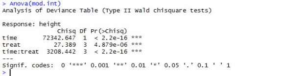
We can see that the main effects of time and treat are highly significant, as is the interaction between the two.

Running a summary() spews out the following log.

As seen,  time:treatF is not  significantly different from the first level , time:treatC , that is, there is no difference between F treatment and C treatment in terms of the interaction with time.Treatments I and IL are significantly different from treatment C in terms of interaction with time.Although there is a significant main effect of treatment, none of the levels are actually different from the first level.

Graphically represented, the affect of time on height, by treatment would like this.

Let’s check the data for adherence to model assumptions.

The plot of residuals versus fitted values doesn’t reflect any obvious pattern in the residuals.So, the assumption of linearity has not been violated and looking at the ‘blob’-like nature of the plot suggests the preservation of Homoskedasticity (One day, I shall pronounce this right).

We’ll check for the assumption of normality of residuals by plotting a histogram. Looks okay to me.

There are several methods for dealing with multicollinearity. In this case, we’ll follow the simplest one, which is to consult the correlation matrix from the output of summary(mod.int) from before. Since none of the correlations between predictors approach 1, we can say that the assumption of  multicollinearity has not been violated.

Moving on.

Bootstrapping is a great resampling technique to arrive at CIs when dealing with mixed effect models where the degree of  various output from them is not clearly known.While one would want to aim  for as high a sampling number as possible to get tighter CIs , we also need to make allowance for longer associated processing times.

So here, we want predictions for all values of height. We will create a test dataset, newdat, which will go as input to predict().

newdat <- subset(tree,treat=="C")
bb <- bootMer(mod.int, FUN=function(x)predict(x, newdat, re.form=NA),
 nsim=999)

#extract the quantiles and the fitted values.
lci <- apply(bb$t, 2, quantile, 0.025)   
uci <- apply(bb$t, 2, quantile, 0.975)   
pred <- predict(mod.int,newdat,re.form=NA)

Plotting the confidence intervals.

library(scales)
palette(alpha(c("blue","red","forestgreen","darkorange"),0.5))
plot(height~jitter(time),col=treat,data=tree[tree$treat=="C",],pch=16)
lines(pred~time,newdat,lwd=2,col="orange",alpha=0.5)
lines(lci~time,newdat,lty=2,col="orange")
lines(uci~time,newdat,lty=2,col="orange")

Conclusion

Using R and lme4 (Bates, Maechler & Bolker, 2012) We performed a linear mixed effects analysis of the relationship between height and treatment of trees, as studied over a period of time. As fixed effects, we entered time and treatment  (with an interaction term) into the model. As random effects, we had intercepts for plotnr (plot numbers). Visual inspection of residual plots did not reveal any obvious deviations from homoscedasticity or normality. P-values were obtained by likelihood ratio tests via anova of the full
model with the effect in question against the model without the effect in question.

. . ..  . and it’s a wrap,folks!

Thanks again for stopping by, and again, I’d be happy to hear your comments and suggestions. Help me make this content better!