
Integration take two – Shiny application
Want to share your content on R-bloggers? click here if you have a blog, or here if you don't.
My last post discussed a technique for integrating functions in R using a Monte Carlo or randomization approach. The mc.int function (available here) estimated the area underneath a curve by multiplying the proportion of random points below the curve by the total area covered by points within the interval:
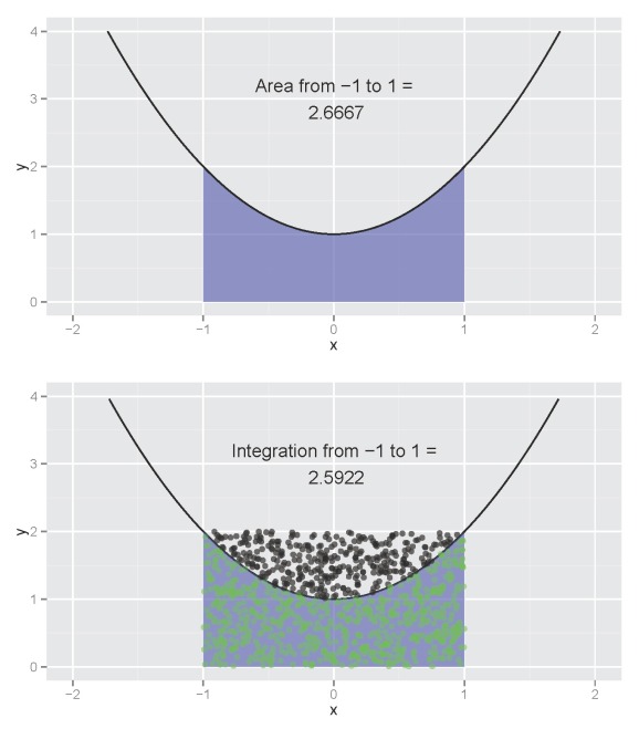
The estimated integration (bottom plot) is not far off from the actual (top plot). The estimate will converge on the actual as the point count reaches infinity. A useful feature of the function is the ability to visualize the integration of a model with no closed form solution for the anti-derivative, such as a loess smooth. I return to the idea of visualizing integrations for this blog using an alternative approach to estimate an integral. I’ve also incorporated this new function using a Shiny interface that allows the user to interactively explore the integration of different functions. I’m quite happy with how it turned out and I think the interface could be useful for anyone trying to learn integration.
The approach I use in this blog estimates an integral using a quadrature or column-based technique (an example). You’ll be familiar with this method if you’ve ever taken introductory calculus. The basic approach is to estimate the integral by summing the area of columns or rectangles that fill the approximate area under the curve. The accuracy of the estimate increases with decreasing column width such that the estimate approaches the actual value as column width approaches zero. An advantage of the approach is ease of calculation. The estimate is simply the sum of column areas determined as width times height. As in my last blog, this is a rudimentary approach that can only approximate the actual integral. R has several methods to more quantitatively approximate an integration, although options for visualization are limited.
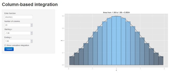
The following illustrates use of a column-based approach such that column width decreases over the range of the interval:
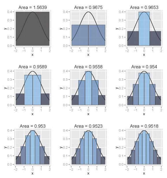
The figure illustrates the integral of a standard normal curve from -1.96 to 1.96. We see that the area begins to approximate 0.95 with decreasing column width. All columns are bounded by the integral and the midpoint of each column is centered on an observed value from the function. The figures were obtained using the column.int function developed for this blog, which can be imported into your workspace as follows:
require(devtools)
source_gist(5568685)
In addition to the devtools package (to import from github), you’ll need to have the ggplot2, scales (which will install with ggplot2), and gridExtra packages installed. You’ll be prompted to install the packages if you don’t have them. Once the function is loaded in your workspace, you can run it as follows (using the default arguments):
column.int()
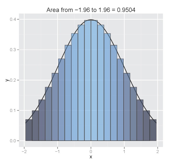
The function defaults to a standard normal curve integrated from -1.96 to 1.96 using twenty columns. The estimated area is projected as the plot title. The arguments for the function as are as follows:
int.fun |
function to be integrated, entered as a character string or as class function, default ‘dnorm(x)’ |
num.poly |
numeric vector indicating number of columns to use for integration, default 20 |
from.x |
numeric vector indicating starting x value for integration, default -1.96 |
to.x |
numeric vector indicating ending x value for integration, default 1.96 |
plot.cum |
logical value indicating if a second plot is included that shows cumulative estimated integration with increasing number of columns up to num.poly, default FALSE |
The plot.cum argument allows us to visualize the accuracy of our estimated integration. A second plot is included that shows the integration obtained from the integrate function (as a dashed line and plot title), as well as the integral estimate with increasing number of columns from one to num.poly using the column.int function. Obviously we would like to have enough columns to ensure our estimate is reasonably accurate.
column.int(plot.cum=T)

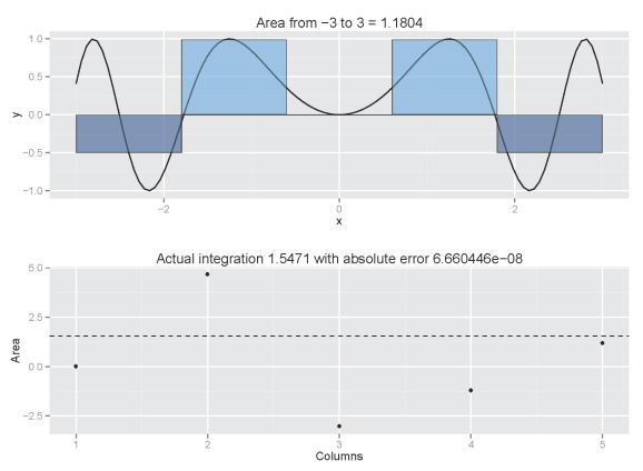
Our estimate converges rapidly to 0.95 with increasing number of columns. The estimated value will be very close to 0.95 with decreasing column width but be aware that computation time increases exponentially. An estimate with 20 columns takes less than a quarter second, whereas an estimate with 1000 columns takes 2.75 seconds. If we include a cumulative plot (plot.cum=T), the processing time is 0.47 seconds for 20 columns and three minutes 37 seconds for 1000 columns. Also be aware that the accuracy of the estimate will vary depending on the function. For the normal function, it’s easy to see how columns provide a reasonable approximation of the integral. This may not be the case for other functions:
column.int('sin(x^2)',n=5,from.x=-3,to.x=3,plot.cum=T)
Increasing the number of columns would be a good idea:
column.int('sin(x^2)',n=100,from.x=-3,to.x=3,plot.cum=T)

Now that you’ve got a feel for the function, I’ll introduce the Shiny interface. As an aside, this is my first attempt using Shiny and I am very impressed with its functionality. Much respect to the creators for making this application available. You can access the interface clicking the image below:
If you prefer, you can also load the interface locally one of two ways:
require(devtools)

shiny::runGist("https://gist.github.com/fawda123/5564846")

shiny::runGitHub('shiny_integrate', 'fawda123')
You can also access the code for the original function below. Anyhow, I hope this is useful to some of you. I would be happy to entertain suggestions for improving the functionality of this tool.
-Marcus
column.int<-function(int.fun='dnorm(x)',num.poly=20,from.x=-1.96,to.x=1.96,plot.cum=F){

	if (!require(ggplot2) | !require(scales) | !require(gridExtra)) {
	  stop("This app requires the ggplot2, scales, and gridExtra packages. To install, run 'install.packages(\"name\")'.\n")
	}

	if(from.x>to.x) stop('Starting x must be less than ending x')

	if(is.character(int.fun)) int.fun<-eval(parse(text=paste('function(x)',int.fun)))

	int.base<-0
	poly.x<-seq(from.x,to.x,length=num.poly+1)

	polys<-sapply(
	  1:(length(poly.x)-1),
		function(i){

			x.strt<-poly.x[i]
			x.stop<-poly.x[i+1]

			cord.x<-rep(c(x.strt,x.stop),each=2)
			cord.y<-c(int.base,rep(int.fun(mean(c(x.strt,x.stop))),2),int.base)
			data.frame(cord.x,cord.y)

			},
		simplify=F
		)

	area<-sum(unlist(lapply(
		polys,
		function(x) diff(unique(x[,1]))*diff(unique(x[,2]))
		)))
	txt.val<-paste('Area from',from.x,'to',to.x,'=',round(area,4),collapse=' ')

	y.col<-rep(unlist(lapply(polys,function(x) max(abs(x[,2])))),each=4)
	plot.polys<-data.frame(do.call('rbind',polys),y.col)

	p1<-ggplot(data.frame(x=c(from.x,to.x)), aes(x)) + stat_function(fun=int.fun)
	if(num.poly==1){
		p1<-p1 + geom_polygon(data=plot.polys,mapping=aes(x=cord.x,y=cord.y),
			alpha=0.7,color=alpha('black',0.6))
		}
	else{
		p1<-p1 + geom_polygon(data=plot.polys,mapping=aes(x=cord.x,y=cord.y,fill=y.col,
			group=y.col),alpha=0.6,color=alpha('black',0.6))
		}
	p1<-p1 + ggtitle(txt.val) + theme(legend.position="none")

	if(!plot.cum) print(p1)

	else{

		area.cum<-unlist(sapply(1:num.poly,
			function(val){
				poly.x<-seq(from.x,to.x,length=val+1)

				polys<-sapply(
				  1:(length(poly.x)-1),
					function(i){

						x.strt<-poly.x[i]
						x.stop<-poly.x[i+1]

						cord.x<-rep(c(x.strt,x.stop),each=2)
						cord.y<-c(int.base,rep(int.fun(mean(c(x.strt,x.stop))),2),int.base)
						data.frame(cord.x,cord.y)

						},
					simplify=F
					)

				sum(unlist(lapply(
					polys,
					function(x) diff(unique(x[,1]))*diff(unique(x[,2]))
					)))

				}
			))

		dat.cum<-data.frame(Columns=1:num.poly,Area=area.cum)
		actual<-integrate(int.fun,from.x,to.x)

		p2<-ggplot(dat.cum, aes(x=Columns,y=Area)) + geom_point()
		p2<-p2 + geom_hline(yintercept=actual$value,lty=2)
		p2<-p2 + ggtitle(paste('Actual integration',round(actual$value,4),'with absolute error',prettyNum(actual$abs.error)))

		grid.arrange(p1,p2)

		}

	}

R-bloggers.com offers daily e-mail updates about R news and tutorials about learning R and many other topics. Click here if you're looking to post or find an R/data-science job.
Want to share your content on R-bloggers? click here if you have a blog, or here if you don't.