Spectral clustering refers to a family of algorithms that cluster eigenvectors derived from the matrix that represents the input data’s graph. An important step in this method is running the kernel function that is applied on the input data to generate a NXN similarity matrix or graph (where N is our number of input observations). Subsequent steps include computing the normalised graph Laplacian from this similarity matrix, getting the eigensystem of this graph, and lastly applying k-means on the top K eigenvectors to get the K clusters. Clustering in this way adds flexibility in the range of data that may be analysed and spectral clustering will often outperform k-means. It is an excellent option for image and bioinformatic cluster analysis including single platform and multi-omics.

‘Spectrum’ is a fast adaptive spectral clustering algorithm for R programmed by myself from QMUL and David Watson from Oxford. It contains both novel methodological advances and implementation of pre-existing methods. Spectrum has the following features; 1) A new density-aware kernel that increases similarity between observations that share common nearest neighbours, 2) A tensor product graph data integration and noise reduction system, 3) The eigengap method to decide on the number of clusters, 4) Gaussian Mixture Modelling for the final clustering of the eigenvectors, 5) Implementation of a Fast Approximate Spectral Clustering method for very big datasets, 6) Data imputation for multi-view analyses. Spectrum has been recently published as an article in Bioinformatics. It is available to download from CRAN: https://cran.r-project.org/web/packages/Spectrum/index.html.

In this demonstration, we are going to use Spectrum to cluster brain cancer RNA-seq to find distinct patient groups with different survival times. This is the link, braincancer_test_data, to download the test data for the analysis. The data can also be accessed through Synapse (https://www.synapse.org/#!Synapse:syn18911542/files/).

## load libraries required for analysis
library(Spectrum)
library(plot3D)
library(survival)
library(survminer)
library(scales)

The next block of code runs Spectrum, then does a t-sne analysis to visualise the clusters embedded in a lower dimensional space.

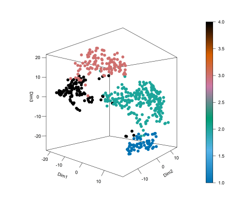
I have found 3D t-sne can work well to see complex patterns of Gaussian clusters which can be found in omic data (as in this cancer data), compared to PCA which is better for a more straightforward structure and outlier detection.

## run Spectrum
r <- Spectrum(brain[[1]])
## do t-sne analysis of results
y <- Rtsne::Rtsne(t(brain[[1]]),dim=3)
scatter3D(y$Y[,1],y$Y[,2],y$Y[,3], phi = 0, #bty = "g", ex = 2,
          ticktype = "detailed", colvar = r$assignments,
          col = gg.col(100), pch=20, cex=2, #type = 'h',
          xlab='Dim1', ylab='Dim2', zlab='Dim3')

Each eigenvector of the graph Laplacian numerically indicates membership of an observation to a block (cluster) in the data's graph Laplacian and each eigenvalue represents how disconnected that cluster is with the other clusters. In the ideal case, if we had eigenvalues reading 1, 1, 1, 1, 0.2 in the below plot, that would tell us we have 4 completely disconnected clusters, followed by one that is much more connected (undesirable when trying to find separate clusters). This principal can be extended to look for the greatest gap in the eigenvalues to find the number of clusters (K).

This first plot, produced automatically by Spectrum of the brain cancer data, shows the eigenvalues for each eigenvector of the graph Laplacian. Here is biggest gap is between the 4th and 5th eigenvectors, thus corresponding to K=4.

This next plot shows the 3D t-sne of the brain cancer RNA-seq clusters. We can see clear separation of the groups. On this type of complex data, Spectrum tends to excel due to its prioritisation of local similarities and its ability to reduce noise by making the k nearest neighbour graph and diffusing on it.

Next, we can run a survival analysis using a Cox proportional hazards model and the log rank test is used to test whether there is a difference between the survival times of different groups (clusters).

## do test
clinicali <- brain[[2]]
clinicali$Death <- as.numeric(as.character(clinicali$Death))
coxFit <- coxph(Surv(time = Time, event = Death) ~ as.factor(r$assignments), data = clinicali, ties = "exact")
coxresults <- summary(coxFit)
print(coxresults$logtest[3])

## survival curve
survival_p <- coxresults$logtest[3]
fsize <- 18
clinicalj <- clinicali
if (0 %in% pr$cluster){
  res$cluster <- res$cluster+1
}
clinicalj$cluster <- as.factor(r$assignments)
fit = survfit(Surv(Time,Death)~cluster, data=clinicalj)

## plot
gg <- ggsurvplot(fit, data = clinicalj, legend = 'right', font.x =  fsize, font.y =  fsize, font.tickslab = fsize,
                 palette = gg.col(4),
                 legend.title = 'Cluster', #3 palette = "Dark2",
                 ggtheme = theme_classic2(base_family = "Arial", base_size = fsize))
gg$plot + theme(legend.text = element_text(size = fsize, color = "black")) + theme_bw() +
  theme(panel.grid.major = element_blank(), panel.grid.minor = element_blank(),
        axis.text.y = element_text(size = fsize, colour = 'black'),
        axis.text.x = element_text(size = fsize, colour = 'black'),
        axis.title.x = element_text(size = fsize),
        axis.title.y = element_text(size = fsize),
        legend.title = element_text(size = fsize),
        legend.text = element_text(size = fsize))

This is the survival curve for the analysis. The code above also gives us the p value (4.03E-22) for the log rank test which is highly significant, suggesting Spectrum yields good results. More extensive comparisons are included in our manuscript.

Spectrum is effective at reducing noise on a single-view (like here) as well as multi-view because it performs a tensor product graph diffusion operation in either case, and it uses a k nearest neighbour graph. Multi-omic clustering examples are included in the package vignette. Spectrum will also be well suited to a broad range of different types of data beyond this demonstration given today.

The density adaptive kernel enhances the intra-cluster similarity which helps to improve the quality of the similarity matrix. A good quality similarity matrix (that represents the data’s graph) is key to the performance of spectral clustering, where intra-cluster similarity should be maximised and inter-cluster similarity minimised.

Spectrum is a fast new algorithm for spectral clustering in R. It is largely based on work by Zelnik-Manor, Ng, and Zhang, and includes implementations of pre-existing methods as well as new innovations. This is the second of the pair of clustering tools we developed for precision medicine, the first being M3C, a consensus clustering algorithm which is on the Bioconductor. In many ways, spectral clustering is a more elegant and powerful method than consensus clustering type algorithms, but both are useful to examine data from a different perspective.

Spectrum can be downloaded here: https://cran.r-project.org/web/packages/Spectrum/index.html

Source code is available here: https://github.com/crj32/Spectrum

Reference

Christopher R John, David Watson, Michael R Barnes, Costantino Pitzalis, Myles J Lewis, Spectrum: fast density-aware spectral clustering for single and multi-omic data, Bioinformatics, , btz704, https://doi.org/10.1093/bioinformatics/btz704