Project Objective

Untappd has some usage restrictions for their API namely not allowing any exploratory of analytics uses, so I’m going to explore tweets of beer and brewery check-ins from the Untappd app to find some implicit trends in how users share their activity.

Exploratory Analysis

library(tidyverse)
library(rtweet)
library(stringr)
library(wesanderson)
library(maps)
library(tidytext)
library(dumas) # http://jasdumas.github.io/dumas/
library(wordcloud)

All social media shares from the Untappd app include their own short URL ‘untp.beer’, which makes the search query criteria identifiable using the search_tweets() function.

untp <- search_tweets(q = "untp.beer", 
                      n = 18000, 
                      include_rts = FALSE, 
                      retryonratelimit = TRUE,  
                      geocode = lookup_coords("usa"), 
                      lang = "en"
)

Let’s take a peek at the text of the tweet!

head(untp$text)

## [1] "I just earned the 'Land of the Free (Level 94)' badge on @untappd! https://t.co/oSOzNMA6tn" 
## [2] "I just earned the 'Wheel of Styles (Level 10)' badge on @untappd! https://t.co/jbW0zjtyAl"  
## [3] "I just earned the 'God Save the Queen' badge on @untappd! https://t.co/CdhKjOKK40"          
## [4] "I just earned the 'Draft City (Level 2)' badge on @untappd! https://t.co/Ps0WOIRUot"        
## [5] "I just earned the 'Middle of the Road (Level 2)' badge on @untappd! https://t.co/XRXVRcc8Iq"
## [6] "Drinking a GRITz by @BrainDeadBrew at @luckdallas — https://t.co/BPCAmDcpdE"

From this sample, its apparent that there a few type of default tweets that are available.

Let’s explore some descriptive stats about the 18,000 tweets that were extracted

How many unique users are in the data set?

length(unique(untp$user_id))

## [1] 5897

paste(min(untp$created_at), max(untp$created_at), sep = " to " )

## [1] "2018-02-04 19:35:40 to 2018-02-05 23:35:29"

My initial assumptions were that all the tweets would be posted from the app, but it seems there is a little bit cross-posting going on from Facebook and some nerds who have set up IFTTT applet recipes.

count(untp, source)

## # A tibble: 3 x 2
##     source     n
##      <chr> <int>
## 1 Facebook    10
## 2    IFTTT     6
## 3  Untappd 17984

How many types of these check-ins are shared?

There a few different types of tweet structures that can be shared from the Untappd app as notices from the text sample above. They include:

1. Earning Badges (i.e. tweets that contain ‘I just earned the…’ or even the word ‘badge’)
2. Added review text (i.e. text which ends in a ‘-‘ before the default template of ‘Drinking a’)
3. Default check-ins (i.e. tweets that begin with ‘Drinking a’)
4. Brewery offering updates (i.e. tweets that begin with ‘Just added …’ for new beers added)

There are granular account social settings available that enable the ease of sharing check-in info to certain linked social media accounts.

I’m going to detect the string patterns and create a new column in the data set to house them.

untp$structure_type <- NA

# earning badges
untp$structure_type[untp$text %>% str_detect("I just earned the")] <- "badge achievement"
# default checkin
untp$structure_type[untp$text %>% str_detect("^Drinking ")] <- "default check-in"
# brewery updates
untp$structure_type[untp$text %>% str_detect("^Just added")] <- "brewery update"
# any NA's left should be tweets that users have added additional text/descriptions
untp$structure_type[is.na(untp$structure_type)] <- "additional review"

Given that a single check-in can result in multiple badges and multiple social shares, this makes sense to have more tweets associated with the type of beer check-in.

untp %>% group_by(structure_type) %>% 
         summarise(n = n()) %>% 
         mutate(structure_type = fct_reorder(structure_type, n)) %>%
    ggplot(., aes(x = structure_type, y = n)) +
      geom_bar(stat = "identity", fill = wes_palette("BottleRocket1", 1)) +
      theme_minimal() +
      labs(title = "Count of Tweet Types for Untappd Twitter Shares", 
           subtitle = "Most users have shared their badge acheivements", y = "Count of Tweets", x = "")

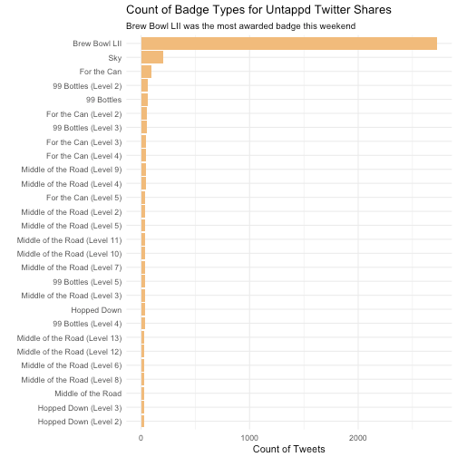
What kind of badges are users earning?

The ‘Brew Bowl LII’ badge is the most popular earned badge available during this Superbowl weekend. Consequently, I visited a brewery this weekend and earned this badge as well.

Drinking a Golden Messenger by @HogRiverBrewing at @hogriverbrewing — https://t.co/70GqltpVXP #photo

— Jasmine Dumas (@jasdumas) February 3, 2018

untp$badge_type <- NA
untp$badge_type <- str_extract(untp$text, "(?<=').*?(?=')")

There were numerous ‘Middle of the Road’ badges awarded of various levels. The description of the Level 5 of that badge is:

Looking for more kick than a session beer, but want to be able to stay for a few rounds? You have to keep it in the middle. That’s 25 beers with an ABV greater than 5% and less than 10%.

So, it would appear that is a popular range of ABV that users are trying, which supports the notion of it’d generally easier to consume more moderate-alcohol content beers rather than heavier beers (Ales vs Stouts).

untp %>% group_by(badge_type) %>% 
         summarise(n = n()) %>% 
         dplyr::filter(!is.na(badge_type)) %>% 
         arrange(desc(n)) %>% 
         top_n(25) %>% 
         mutate(badge_type = fct_reorder(badge_type, n)) %>%
    ggplot(., aes(x = badge_type, y = n)) +
      geom_bar(stat = "identity", fill = wes_palette("GrandBudapest1", 1)) +
      theme_minimal() +
      coord_flip() +
      labs(title = "Count of Badge Types for Untappd Twitter Shares", 
           subtitle = "Brew Bowl LII was the most awarded badge this weekend", y = "Count of Tweets", x = "")

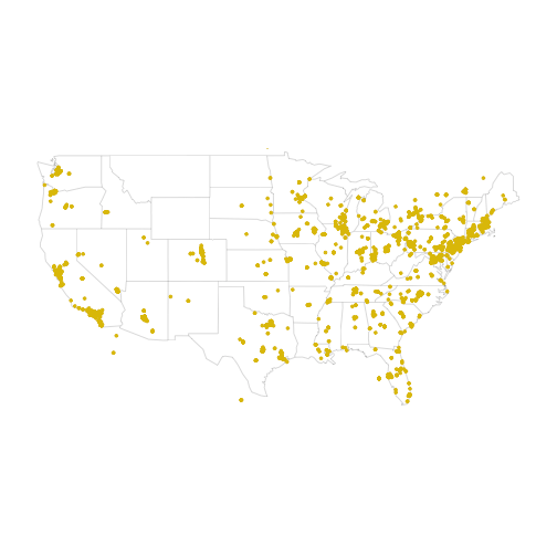
Where do people check-in from?

Lot’s of activity on the east coast (Boston, MA being the top place at the time of running this analysis) and in the metros across the U.S.! Untappd is based in North Carolina, so it’s interesting to not see a lot of activity there, but users can have their location settings turned off for privacy in Twitter. This may also be indicative of users not filling out all the check-in details such as purchase or drinking location. Often times users seem to be drinking and checking-in at home and may want to mask their location given the plethora of missing values.

untp %>% group_by(place_full_name) %>% 
  summarise(n = n()) %>% 
  arrange(desc(n)) %>% 
  top_n(11) %>% 
  data.frame()

##       place_full_name     n
## 1                <NA> 14776
## 2   Pennsylvania, USA    81
## 3        Florida, USA    66
## 4        Portland, OR    62
## 5  Cape Girardeau, MO    44
## 6    Philadelphia, PA    38
## 7         Phoenix, AZ    36
## 8          Dallas, TX    34
## 9     Los Angeles, CA    34
## 10       Brooklyn, NY    33
## 11      New York, USA    33

There are a few off the map, but the general distribution is effectively visualized with one yellow dot per tweet.

## create lat/lng variables using all available tweet and profile geo-location data
untp <- lat_lng(untp)

## plot state boundaries
par(mar = c(0, 0, 0, 0))
maps::map("state", lwd = .25)

## plot lat and lng points onto state map
with(untp, points(lng, lat, pch = 20, cex = .75, col = wes_palette("Cavalcanti1", 1)))

What are the most popular breweries?

Instead of crafting an ugly regex solution to extract the brewery from the tweet text, the column for mentions_screen_name is actually a decent proxy for the beer location if the brewery has a Twitter presence! I really enjoy Tree House Brewery, Green IPA and it is nice to see many others have tried out beers from their brewery.

# mentions_screen_name is the brewery that produced the checked-in beer
tibble(brewery = unlist(untp$mentions_screen_name)) %>% 
        group_by(brewery) %>% 
        dplyr::filter(brewery != 'untappd') %>% 
        summarise(n = n()) %>% 
        arrange(desc(n)) %>% 
        top_n(25) %>% 
  mutate(brewery = fct_reorder(brewery, n)) %>%
    ggplot(., aes(x = brewery, y = n)) +
      geom_bar(stat = "identity", fill = wes_palette("Moonrise2", 1)) +
      theme_minimal() +
      coord_flip() +
      labs(title = "Top 25 Breweries for Untappd Twitter Shares", 
           subtitle = "", y = "Count of Tweets", x = "", caption = "by @handle occurrences")

How many pictures of beer are shared?

The #photo is indicative of a paired photo with a tweet from Untappd. The rest of the hash tags align with the Superbowl festivities

tibble(hashtags = unlist(untp$hashtags)) %>% 
        group_by(hashtags) %>% 
        dplyr::filter(!is.na(hashtags)) %>% 
        summarise(n = n()) %>% 
        arrange(desc(n)) %>% 
        top_n(25)

## # A tibble: 25 x 2
##                hashtags     n
##                   <chr> <int>
##  1                photo  2897
##  2             brewbowl  2728
##  3        ibelieveinIPA    62
##  4            SuperBowl    40
##  5         FlyEaglesFly    37
##  6         FirstSqueeze    26
##  7            craftbeer    21
##  8 BrainDeadBottleShare    16
##  9          beerandfood    15
## 10        UntapTheStack    15
## # ... with 15 more rows

Did people share more during the Superbowl game?

There was definitely a spike on Sunday as the Superbowl was starting!

## plot time series of tweets
ts_plot(untp, "1 hours") +
  ggplot2::theme_minimal() +
  ggplot2::theme(plot.title = ggplot2::element_text(face = "bold")) +
  ggplot2::labs(
    x = NULL, y = NULL,
    title = "Frequency of Untappd Twitter statuses from the past 2 days",
    subtitle = "Twitter status (tweet) counts aggregated using one-hour intervals",
    caption = "\nSource: Data collected from Twitter's REST API via rtweet"
  )

Sentiment Analysis

We want to separate all the text before the dash (-) which is how the tweet is structured when users add additional text to their beer review share.

# the first vector is the review, second is the beer/brewery, third is the url
untp_text <- str_split(untp$text[untp$structure_type == 'additional review'], "-|—")

# unnest these unnamed lists, if they were named I would have used purrr::map_df()
# https://stackoverflow.com/a/24496537/4143444
review <- sapply(untp_text, "[", 1)
beer <- sapply(untp_text, "[", 2)
user <-untp %>% 
        dplyr::filter(structure_type == 'additional review') %>% 
        select(starts_with("screen_name"))
untp_text <- data.frame(review, beer, user$screen_name)

Let’s remove the hash tags from the beer column and the common begging of each description.

untp_text$clean_beer <- str_replace(untp_text$beer,"#[a-zA-Z0-9]{1,}", "")

untp_text$clean_beer <- str_replace_all(untp_text$clean_beer, c("Drinking a |Drinking an "), "") 

untp_text$clean_beer <- str_replace_all(untp_text$clean_beer, "[[:punct:]]", "") 

untp_text$clean_beer <- trimws(untp_text$clean_beer)

Now that we have the reviews and beer/breweries separated, I wonder if there are any commonly reviewed beers that are shared on Twitter? (I want to keep the beer with the brewery at this point in case the same beer name appears at different breweries)

untp_text %>% group_by(clean_beer) %>% 
              summarise(n = n()) %>% 
              arrange(desc(n)) %>% 
              top_n(15) %>% 
              dplyr::filter(clean_beer %notin% c("DC", "A")) %>% 
  mutate(clean_beer = fct_reorder(clean_beer, n)) %>%
    ggplot(., aes(x = clean_beer, y = n)) +
      geom_bar(stat = "identity", fill = wes_palette("BottleRocket2", 1)) +
      theme_minimal() +
      coord_flip() +
      labs(title = "Top 15 Beers for Untappd\nTwitter Shares", 
           subtitle = "", y = "Count of Tweets", x = "")

Translating the additional review text as proxy for empirical reviews

These tweets don’t indicate what numerical value that users rated each beer on a scale of 0.0 to 5.0 (0.25 increments) on the app, so I’m going to try and derive some of users opinions about beer from tweets that have additional review text, using the tidytext package. I think there is going to be some sentiment shared that is linked to the Super Bowl, and some selection bias from user’s most likely sharing preferred beers.

top_beers <- untp_text %>% group_by(clean_beer) %>% 
              summarise(n = n()) %>% 
              arrange(desc(n)) %>% 
              top_n(20) %>% 
              dplyr::filter(clean_beer %notin% c("DC", "A")) %>% 
              select(clean_beer)

# subset the data into topic (beers) and review (text) for tokenization
untp_text_tiny <- untp_text[, c("clean_beer", "review")]

# need to inner_join top beers with the reviews
merge_untp <- untp_text_tiny %>% 
              inner_join(top_beers)

# tokenize the reviews and remove some of the specific football words
untp_text_tiny <- merge_untp %>% 
                  unnest_tokens(word, review) %>% 
                  dplyr::filter(word %notin% c("super", "superbowl", "superbowlsunday"
))

untp_sentiment <- 
  untp_text_tiny %>%
    inner_join(get_sentiments("bing")) %>%
    count(clean_beer, sentiment) %>%
    spread(sentiment, n, fill = 0) %>%
    mutate(sentiment = positive - negative) 

head(untp_sentiment)

## # A tibble: 6 x 4
##                                             clean_beer negative positive
##                                                  <chr>    <dbl>    <dbl>
## 1                                    6 by relicbrewing        0        2
## 2                                  Abbey by newbelgium        0        3
## 3                                               Barrel        3        4
## 4                                       Bourbon Barrel        2        2
## 5            Bourbon County Brand Stout by GooseIsland        0        2
## 6 Canadian Breakfast Stout CBS 2017 by foundersbrewing        0        2
## # ... with 1 more variables: sentiment <dbl>

The ‘Drifter Pale Ale Widmer Brothers Brewing’ having the lowest associated sentiment and currently rated: 3.43 and the ‘Stone Delicious IPA by Stone Brewing’ having the highest associated sentiment which is currently rated: 3.81.

ggplot(untp_sentiment, aes(x = clean_beer, y = sentiment, fill = clean_beer)) +
  geom_col(show.legend = FALSE) +
  coord_flip() +
  theme_minimal() +
  labs(x = "")

Now, I want to visualize the words to see the most common occurrences from added reviews. The largest word being ‘Beer’ is the most obvious given the specific Untappd reviews. Then the other words appear to be popular hash tags from the Superbowl such as ‘flyeaglesfly’.

untp_text_tiny %>%
  anti_join(stop_words) %>%
  count(word) %>%
  with(wordcloud(word, n, max.words = 100, colors = wes_palette("Zissou1")))

Notes:

1. Untappd has a supporter program which comes with a feature for downloading your personal check-in data.

2. I did not intentionally set out to run this analysis during the Superbowl and I did not watch the game!