Calibrated Hull and White short-rates with RQuantLib and ESGtoolkit
Want to share your content on R-bloggers? click here if you have a blog, or here if you don't.
In this post, I use R packages RQuantLib and ESGtoolkit for the calibration and simulation of the famous Hull and White short-rate model.
QuantLib is an open source C++ library for quantitative analysis, modeling, trading, and risk management of financial assets. RQuantLib is built upon it, providing R users with an interface to the library .
ESGtoolkit provides tools for building Economic Scenarios Generators (ESG) for Insurance. The package is primarily built for research purpose, and comes with no warranty. For an introduction to ESGtoolkit, you can read this slideshare, or this blog post. A development version of the package is available on Github with, I must admit, only 2 or 3 commits for now.
The Hull and White (1994) model was proposed to address Vasicek’s model poor fitting of the initial term structure of interest rates. The model is defined as:
Where and
are positive constants, and
is a standard brownian motion under a risk-neutral probability.
, which is constant in Vasicek’s model, is a function constructed so as to correctly match the initial term structure of interest rates.
An alternative and convenient representation of the model is:
where
and are market-implied instantaneous forward rates for maturities
.
In insurance market consistent pricing, the model is often calibrated to swaptions, as there are no market prices for embedded options and guarantees.
Two parameters and
are surely not enough to get back the whole swaptions volatility surface (or even ATM swaptions). But a perfect calibration to market-quoted swaptions isn’t vital and may lead to unnecessary overfitting. A more complex model may fit more precisely the swaptions volatility surface, but could still be proved to be more wrong for the purpose: insurance liabilities do not even match exactly market swaptions’ characteristics.
It’s worth mentioning that the yield curve bootstrapping procedure currently implemented in RQuantLib, makes the implicit assumption that LIBOR is a good proxy for risk-free rates, and collateral doesn’t matter. These assumptions are still widely used in insurance, along with simple (parallel) adjustments for credit/liquidity risks, but were abandoned by markets after the 2007 subprime crisis.
For more details on the new multiple-curve approach, see for example http://papers.ssrn.com/sol3/papers.cfm?abstract_id=2219548. In this paper, the authors introduce a multiple-curve bootstrapping procedure, available in QuantLib.
# Cleaning the workspace
rm(list=ls())

# RQuantLib loading
suppressPackageStartupMessages(library(RQuantLib))
# ESGtoolkit loading
suppressPackageStartupMessages(library(ESGtoolkit))

# Frequency of simulation and interpolation
freq <- "monthly"
delta_t <- 1/12

# This data is taken from sample code shipped with QuantLib 0.3.10.
params <- list(tradeDate=as.Date('2002-2-15'),
               settleDate=as.Date('2002-2-19'),
               payFixed=TRUE,
               dt=delta_t,
               strike=.06,
               method="HWAnalytic",
               interpWhat="zero",
               interpHow= "spline")

# Market data used to construct the term structure of interest rates
# Deposits and swaps
tsQuotes <- list(d1w =0.0382,
                 d1m =0.0372,
                 d3m = 0.0363,
                 d6m = 0.0353,
                 d9m = 0.0348,
                 d1y = 0.0345,
                 s2y = 0.037125,
                 s3y =0.0398,
                 s5y =0.0443,
                 s10y =0.05165,
                 s15y =0.055175)

# Swaption volatility matrix with corresponding maturities and tenors
swaptionMaturities <- c(1,2,3,4,5)
swapTenors <- c(1,2,3,4,5)
volMatrix <- matrix(
  c(0.1490, 0.1340, 0.1228, 0.1189, 0.1148,
    0.1290, 0.1201, 0.1146, 0.1108, 0.1040,
    0.1149, 0.1112, 0.1070, 0.1010, 0.0957,
    0.1047, 0.1021, 0.0980, 0.0951, 0.1270,
    0.1000, 0.0950, 0.0900, 0.1230, 0.1160),
  ncol=5, byrow=TRUE)

# Pricing the Bermudan swaptions
pricing <- RQuantLib::BermudanSwaption(params, tsQuotes,
                            swaptionMaturities, swapTenors, volMatrix)
summary(pricing)

# Constructing the spot term structure of interest rates
# based on input market data
times <- seq(from = delta_t, to = 5, by = delta_t)
curves <- RQuantLib::DiscountCurve(params, tsQuotes, times)
maturities <- curves$times
marketzerorates <- curves$zerorates
marketprices <- curves$discounts

############# Hull-White short-rates simulaton

# Horizon, number of simulations, frequency
horizon <- 5 # I take horizon = 5 because of swaptions maturities
nb.sims <- 10000

# Calibrated Hull-White parameters from RQuantLib
a <- pricing$a
sigma <- pricing$sigma

# Simulation of gaussian shocks with ESGtoolkit
set.seed(4)
eps <- ESGtoolkit::simshocks(n = nb.sims, horizon = horizon,
                             frequency = freq)

# Simulation of the factor x with ESGtoolkit
x <- ESGtoolkit::simdiff(n = nb.sims, horizon = horizon,
                         frequency = freq,
                         model = "OU",
                         x0 = 0, theta1 = 0,
                         theta2 = a,
                         theta3 = sigma,
                         eps = eps)

# I use RQuantlib's forward rates. With the low monthly frequency,
# I consider them as being instantaneous forward rates
fwdrates <- ts(replicate(nb.sims, curves$forwards),
                start = start(x),
                deltat = deltat(x))

# alpha
t.out <- seq(from = 0, to = horizon, by = delta_t)
param.alpha <- ts(replicate(nb.sims, 0.5*(sigma^2)*(1 - exp(-a*t.out))^2/(a^2)),
                start = start(x), deltat = deltat(x))
alpha <- fwdrates + param.alpha

# The short-rate
r <- x + alpha

# Stochastic discount factors (numerical integration currently is very basic)
Dt <- ESGtoolkit::esgdiscountfactor(r = r, X = 1)

# Monte Carlo prices and zero rates deduced from stochastic discount factors
montecarloprices <- rowMeans(Dt)
montecarlozerorates <- -log(montecarloprices)/maturities # RQuantLib uses continuous compounding

# Confidence interval for the difference between market and monte carlo prices
conf.int <- t(apply((Dt - marketprices)[-1, ], 1, function(x) t.test(x)$conf.int))

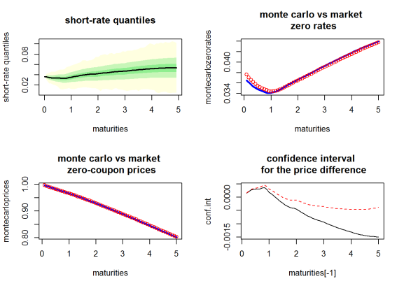
# Viz
par(mfrow = c(2, 2))
# short-rate quantiles
ESGtoolkit::esgplotbands(r, xlab = "maturities", ylab = "short-rate quantiles",
                         main = "short-rate quantiles")
# monte carlo vs market zero rates
plot(maturities, montecarlozerorates, type='l', col = 'blue', lwd = 3,
     main = "monte carlo vs market n zero rates")
points(maturities, marketzerorates, col = 'red')
# monte carlo vs market zero-coupon prices
plot(maturities, montecarloprices, type ='l', col = 'blue', lwd = 3,
     main = "monte carlo vs market n zero-coupon prices")
points(maturities, marketprices, col = 'red')
# confidence interval for the price difference
matplot(maturities[-1], conf.int, type = 'l',
        main = "confidence interval n for the price difference")
R-bloggers.com offers daily e-mail updates about R news and tutorials about learning R and many other topics. Click here if you're looking to post or find an R/data-science job.
Want to share your content on R-bloggers? click here if you have a blog, or here if you don't.

