Bayesian Simple Linear Regression with Gibbs Sampling in R

Posted on August 7, 2017 by Arman Oganisian in R bloggers | 0 Comments

[This article was first published on R – Stable Markets, and kindly contributed to R-bloggers]. (You can report issue about the content on this page here)

Want to share your content on R-bloggers? click here if you have a blog, or here if you don't.

Many introductions to Bayesian analysis use relatively simple didactic examples (e.g. making inference about the probability of success given bernoulli data). While this makes for a good introduction to Bayesian principles, the extension of these principles to regression is not straight-forward.

This post will sketch out how these principles extend to simple linear regression. Along the way, I will derive the posterior conditional distributions of the parameters of interest, present R code for implementing a Gibbs sampler, and present the so-called grid point method.

I’ve had trouble with R code snippets in wordpress before, so I will not present code in the post. Instead, I’ll host the code on GitHub. You can follow along with the code as you go through the post.

A Bayesian Model

Suppose we observe data $(y_i, x_i)$ for $i \in \{1, \dots, n \}$ . Our model for $y$ is

$y_i \sim N(\beta_0 + \beta_1 x_i, \phi )$

Of interest is making inference about $\beta_0$ and $\beta_1$ . If we place normal priors on the coefficients and an inverse gamma prior on the variance term, the full bayesian model for this data can be written as:

$y_i | \beta_0, \beta_1, \phi \sim N(\beta_0 + \beta_1 x_i, \phi )$
$\beta_0 | \mu_0, \tau_0 \sim N(\mu_0, \tau_0)$
$\beta_1 | \mu_1, \tau_1 \sim N(\mu_1, \tau_1)$
$\phi | \alpha, \gamma \sim IG(\alpha, \gamma)$

Assuming the hyperparameters $\mu_0, \tau_0, \mu_1, \tau_1, \alpha$ and $\gamma$ are known, the posterior can be written up to a constant of proportionality,

$p(\beta_0, \beta_1, \phi | \vec y) \propto \Big [\prod_{i=1}^n p(y_i | \beta_0, \beta_1, \phi )\Big] p( \beta_0 | \mu_0, \tau_0 ) p(\beta_1 | \mu_0, \tau_0) p( \phi | \alpha, \gamma)$

The term in the brackets is the joint distribution of the data, or likelihood. The other terms comprise the joint prior distribution of the parameters (since we implicitly assumed prior independence, the joint prior factors).

This is recognized as the familiar expression:

$posterior \propto likelihood \times prior$ .

Part 0 of the accompanying R code generates data from this model for specified “true” parameters. We will later estimate a bayesian regression model with this data to check that we can recover these true parameters.

The Gibbs Sampler

To draw from this posterior distribution, we can use the Gibbs sampling algorithm. Gibbs sampling is an iterative algorithm that produces samples from the posterior distribution of each parameter of interest. It does so by sequentially drawing from the conditional posterior of the each parameter in the following way:

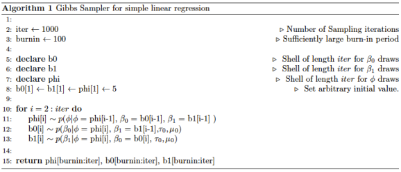
It can be shown that, after a suitable burn-in period, the remaining of the 1,000 draws are draws from the posterior distributions. These samples are not independent. The sequence of draws is a random walk in the posterior space and each step in the space depends on the previous position. Typically a thinning period will also be used (which is not done here). A thinning of 10 would mean that we keep every 10th draw. The idea being that each draw may be dependent on the previous draw, but not as dependent on the 10th previous draw.

Conditional Posterior Distributions

To use Gibbs, we need to identify the conditional posterior of each parameter.

It helps to start with the full unnormalized posterior:

$p(\beta_0, \beta_1, \phi | \vec y) \propto \phi^{-n/2} e^{-\frac{1}{2\phi} \sum_{i=1}^{n}(y_i - (\beta_0 + \beta_1x_i) )^2 } e^{-\frac{1}{2\tau_0} (\beta_0 - \mu_0 )^2 } e^{-\frac{1}{2\tau_1} (\beta_1 - \mu_1 )^2 } \phi^{-(\alpha + 1) e^{-\frac{\gamma}{\phi}}}$

To find the conditional posterior of a parameter, we simply drop all terms from the joint posterior that do not include that parameter. For example, the constant term $\beta_0$ has conditional posterior:

$p(\beta_0 | \phi,\beta_1, \mu_0, \tau_0, \vec y) \propto e^{-\frac{1}{2\phi} \sum_{i=1}^n (y_i - (\beta_0 + \beta_1x_i) )^2 } e^{-\frac{1}{2\tau_0} (\beta_0 - \mu_0 )^2 }$

Similarly,

$p(\beta_1 | \beta_0, \phi, \mu_1, \tau_1, \vec y) \propto e^{-\frac{1}{2\phi} \sum_{i=1}^{n}(y_i - (\beta_0 + \beta_1x_i) )^2 } e^{-\frac{1}{2\tau_1} (\beta_1 - \mu_1 )^2 }$

The conditional posterior can be recognized as another inverse gamma distribution, with some algebraic manipulation.

$\begin{aligned} p(\phi | \beta_0, \beta_1, \alpha, \gamma, \vec y) & \propto \phi^{-n/2} \phi^{-(\alpha + 1) e^{-\frac{\gamma}{\phi}}} e^{-\frac{1}{2\phi} \sum_{i=1}^{n}(y_i - (\beta_0 + \beta_1x_i) )^2} \\ & = \phi^{-(\alpha + \frac{n}{2} + 1)} exp{-\frac{1}{\phi} \Big[ \frac{1}{2\phi} \sum_{i=1}^{n}(y_i - (\beta_0 + \beta_1x_i) )^2 + \gamma \Big] } \\ & = IG(shape = \alpha + \frac{n}{2}, \ rate = \frac{1}{2\phi} \sum_{i=1}^{n}(y_i - (\beta_0 + \beta_1x_i) )^2 + \gamma ) \end{aligned}$

The conditional posteriors of $\beta_0$ and $\beta_1$ aren’t as easy to recognize. But we don’t really need to go through any algebra if we’re willing ot use the grid method.

The Grid Method

Consider $\beta_0$ . The grid method is a very brute force way (in my opinion) to sample from its conditional posterior distribution. This conditional distribution is just a function of $\beta_0$ . So we can evaluate the density for certain $\beta_0$ values. In R notation, this can be grid=seq(-10, 10, by=.001), say. This sequence is the “grid” of points.

Then the conditional posterior distribution evaluated at each grid point tells us the relatively likelihood of that draw.

We can then use the sample() function in R to draw from these grid of points, with sampling probabilities proportional to the density evaluation at the grid points.

This is implemented in functions rb0cond() and rb1cond() in part 1 of the accompanying R code.

It is common to encounter numerical issues when using the grid method. Since we are evaluating an unnormalized posterior on the grid, the results can get quite large or small. This may yield Inf and -Inf values in R.

In functions rb0cond() and rb1cond(), for example, I actually evaluate the log of the conditional posterior distributions derived. I then normalize by subtracting each evaluation from the maximum of all the evaluations before exponentiating back from the log scale. This tends to handle such numerical issues.

We don’t need to use the grid method to draw from the conditional posterior of $\phi$ since it is from a known distribution.

Note that this grid method has some drawbacks.

First, it’s computationally expensive. It would be more computationally efficient to go through the algebra and hopefully get a known posterior distribution to draw from, as we did with $\phi$ .

Second, the grid method requires specifying a region of grid points. What if the conditional posterior had significant density outside our specified grid interval of [-10,10]? In this case, we would not get an accurate sample from the conditional posterior. It’s important to keep this in mind and experiment with wide grid intervals. So, we need to be clever about handling numerical issues such as numbers approaching Inf and -Inf values in R.

Simulation Results

Now that we have a way to sample from each parameter’s conditional posterior, we can implement the Gibbs sampler. This is done in part 2 of the accompanying R code. It codes the same algorithm outlined above in R.

The results are good. The plot below shows the sequence of 1000 Gibbs samples (with burn-in draws removed and no thinning implemented). The red lines indicate the true parameter values under which we simulate the data. The fourth plot shows the joint posterior of the intercept and slope terms, with red lines indicating contours.

To sum things up, we first derived an expression for the joint distribution of the parameters. Then we outlined the Gibbs algorithm for drawing samples from this posterior. In the process, we recognized that the Gibbs method relies on sequential draws from the conditional posterior distribution of each parameter. For $\phi$ , this was an easily recognized, known distribution. For the slope and intercept terms, we decided to circumvent the algebra by using the grid method. This benefits of doing this is that we side step a lot of algebra. The costs are increased computational complexity, some trial and error when choosing appropriate range for the grid, and numerical issues.

I’ll try to follow up with an extension to a bayesian multivariate linear regression model in the near future.

To leave a comment for the author, please follow the link and comment on their blog: R – Stable Markets.

R-bloggers.com offers daily e-mail updates about R news and tutorials about learning R and many other topics. Click here if you're looking to post or find an R/data-science job.

Want to share your content on R-bloggers? click here if you have a blog, or here if you don't.

R-bloggers

R news and tutorials contributed by hundreds of R bloggers

Bayesian Simple Linear Regression with Gibbs Sampling in R

A Bayesian Model

The Gibbs Sampler

Conditional Posterior Distributions

The Grid Method

Simulation Results

Related

A Bayesian Model

The Gibbs Sampler

Conditional Posterior Distributions

The Grid Method

Simulation Results

Related

Never miss an update! Subscribe to R-bloggers to receive e-mails with the latest R posts. (You will not see this message again.)

Never miss an update!
Subscribe to R-bloggers to receive
e-mails with the latest R posts.
(You will not see this message again.)