1. Visualizing Data

1. R Programming
2. Text Mining
3. WordCloud

Having state election coming soon in Victoria (Australian state where I live) I decided to make a quick analysis and compare what politicians from major Australian party’s post in their Twitter accounts.

I have collected Twitter hanldes of Australian Parliament members (also referred in text and code as MP that states for Member of Parliament) grouped by party. If you are interested how I did it using RSelenium you are welcome to check it in my blog post.

Now I'll use this dataset to collect tweets and do a quick analysis. Start from loading required libraries and the dataframe with Twitter handles.

library(dplyr)
library(purrr)
library(twitteR)
#load dataset from CSV file
mps <- read.csv('mps.csv')

Filter out MPS without Twitter accounts and smaller parties and separate it to different objects

majors <- c("Australian Labor Party", "Liberal Party of Australia", "The Nationals")
mp2 <- mps %>% filter(twitter!="NA" & party %in% majors) %>% group_by(party)
labor <- mp2 %>% filter(party=="Australian Labor Party")
libs <- mp2 %>% filter(party=="Liberal Party of Australia")
nationals <- mp2 %>% filter(party=="The Nationals")

No lets check number of accounts per party

mp2 %>% summarise(n = n())
## # A tibble: 3 x 2
##   party                          n
##   <fct>                      <int>
## 1 Australian Labor Party        48
## 2 Liberal Party of Australia    37
## 3 The Nationals                  9

Looks correct. So we can start using Twitter API to collect the data. There is a handy package for R called TwitterR that we alreay loaded.
If you don't have an app registered in Twitter you need one. You can do it at Twitter Developer website

## download cert file
download.file(url = "http://curl.haxx.se/ca/cacert.pem",
              destfile = "cacert.pem")

# You need your own API key in format
# apikeys <- c ('YOU API KEY', # api key
#               'YOUR API SECRET', # api secret
#               'YOU API ACCESS TOKEN', # access token
#               'YOUR API SECRET TOKEN') # access token secret)
# 
source("api_key.r") #local file as per the structue above, you need to create your own
setup_twitter_oauth(apikeys[1], apikeys[2],apikeys[3], apikeys[4])

You may be asked to prompt saying “Use a local file to cache OAuth access credentials between R sessions?, where you should answer Yes. If you getting errors try to install or update openssl package.

Now define own search function based on, conduct the search and save the results so, can use it later

tsearch <- function (username, n=100){
        q=paste0('from:',as.character(username))
        result <-searchTwitter(q, resultType="recent", n=n, retryOnRateLimit=5)
        return(result)
}
# collecting tweets 
tweets_nat <- map(nationals$twitter, ~tsearch(.x, n=200))
tweets_lab<- map(labor$twitter, ~tsearch(.x, n=200))
tweets_lib<- map(libs$twitter, ~tsearch(.x, n=200))
## we need the last 3 objetcs in analysis script
save(tweets_nat, tweets_lab, tweets_lib, file = "tweets.RData")

Data collection is done. We can move to data analysis.

Data analysis

Good way to have quick outlook to text data is to use word clouds. Let’s build them!

Load several libraries

require(stringr)
require(tm)
require(wordcloud)
require(SnowballC)

Load data – tweets we collected and prepare it for building word clouds

load("tweets.Rdata")
# Function to extract text only 
gettext<- function (mylist) {
        text <- character()
        for (i in 1:length(mylist)){
        text <- append(text,  mylist[[i]][[".->text"]])        
        }
        return(text)        
}
# for some reasons unlist inside function doesn't work, so sample call should look like
text <- gettext(unlist(tweets_nat))

Next we'll build text corpus (here tm package functionality used, SnowballC used for stemming). To be honest stemming result is a bit clunky, you may see words like 'communiti' or 'minist' that probably coming from there. So if you know better stemming approach – I'll appreciate a reference.

# build and clean corpus
corp <- function (text) {
        text_df <- data_frame(line = 1, text = text)     
        # clean up some stuff
        text_df <- sapply(text_df$text,function(row) iconv(row, "latin1", "ASCII", sub=""))
        #corpus is a collection of text documents
        t_corpus <- Corpus(VectorSource(text_df))
        #clean text and stemming
        t_clean <- tm_map(t_corpus, removePunctuation)
        t_clean <- tm_map(t_clean, content_transformer(tolower))
        t_clean <- tm_map(t_clean, removeWords, stopwords("english"))
        t_clean <- tm_map(t_clean, removeNumbers)
        t_clean <- tm_map(t_clean, stripWhitespace)
        t_clean <- tm_index(t_clean, stemDocument)
        return(t_clean)        
}

lab_corp <- gettext(unlist(tweets_lab)) %>% corp()
lib_corp <- gettext(unlist(tweets_lib)) %>% corp()
nat_corp <- gettext(unlist(tweets_nat)) %>% corp()

Now we can start building word clouds.
First define own function with nicer than default formatting.

mywordcloud <- function (corp) {
        wc <-wordcloud(corp, random.order=F,max.words=80, col=rainbow(80), scale=c(3,0.2))        
        return(wc)
}

Next we'll build wordclouds for all parties.

Labor

plot.new()
lab_wc <- lab_corp %>% mywordcloud()

Liberals

plot.new()
lib_wc <- lib_corp %>% mywordcloud()

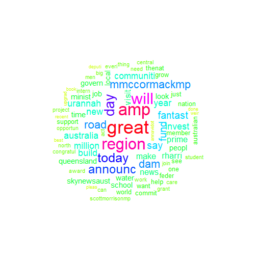
Nationals

plot.new()
nat_wc <- nat_corp %>% mywordcloud()

Commonality and differences

We can also check what is common in different between content of Twitter posts of different parties. First, we need wrange the data a bit

## Reducing dimensions - one document per party

# defining function
my_tm <- function (corp, name){
        term.matrix <- termFreq (corp) %>% as.matrix() 
        colnames(term.matrix)<- name
        # transpose to merge later
        #term.matrix <- t(term.matrix)
        term.matrix <- as.data.frame(term.matrix)
        term.matrix$word <- row.names(term.matrix)
        return(term.matrix)
}
# to new df
atm_nats <-  my_tm (nat_corp, "Nationals")
atm_libs <-  my_tm (lib_corp, "Liberals")
atm_labs <-  my_tm (lab_corp, "Labor")
# join
atm <- full_join(atm_nats, atm_libs, by = 'word') %>% full_join(atm_labs,by = 'word')
# formatting for further use
row.names(atm)<-atm$word
atm <- atm[c(1,3,4)]
atm <- as.matrix(atm)
atm[is.na(atm)] <- 0

Next we can build comparison word cloud and commonality cloud

Comparison word cloud

# Comparison Cloud, words that are party specific
plot.new()
comparison.cloud(atm,max.words=80,scale=c(3,.2), random.order=FALSE, colors=brewer.pal(max(3,ncol(atm)),"Dark2"),
                 use.r.layout=FALSE, title.size=3,
                 title.colors=NULL, match.colors=FALSE,
                 title.bg.colors="grey90")

Commonality word cloud

plot.new()
commonality.cloud(atm, max.words=80,random.order=FALSE)     

Quick observations

You may do your own analysis of the results, but there are several things that I've noticed:

• All parties use 'will' and 'great' and 'Australia' a lot, probably talking about great things that they will do in the future for our country ????
• Naturally all MPs often refer party leaders to party leaders (Bill Shorten, Scott Morrison and Michael McCormack). What is interesting that Scott Morison much more often referred by Labor than Bill Shorten by Liberals.
• Rather than referring party leader, Liberals prefer to talk much more about 'Labor' as party.
• Nationals talk much more about regions – their 9 MPs with Twitter accounts generated over twice as much posts with this keyword as combined ALP (48) and Liberal (37) MPs.
• Interesting that Labor used word 'tax' twice as often as Liberals
• I was surprised to see so many tweets with 'amp' and thought that it is about AMP (financial institution). Appeared that it was formatting used, so i should clean it out.

Full source code and resulting files can be found in Github repository

1. Introducing vizscorer: a bot advisor to score and improve your ggplot plots
2. Visualize your CV’s timeline with R (Gantt chart style)
3. Analysing UK Traffic Trends with PCA
4. Time series visualizations with wind turbine energy data in R
5. Visualizations for credit modeling in R