
24 Days of R: Day 13
In this post, I'll look at a very quick way to look at the relationships in a database. I had a bit of fun with my first network graph and plotting the connections between tables and views seems like a natural extension. Here, I'm going to create a bare bones insurance database. We have a defined business segment, which contains one or more accounts. Each account purchases one or more policies and each policy has one or more claims. Finally, each claim is evaluated over the course of its existence and paid and outstanding losses are recorded. Very basic. I'm not going to describe the schema here (though you can see it on my GitHub at the RxR project). The point is to explore the structure of a database without knowing anything at all about it.
I'm using (free, but closed source) SQL Server Compact as I'm having difficulty getting the PostgreSQL ODBC driver to play nicely with RODBC. I've just started diagnosing this- it's almost certainly a 32 vs. 64 bit issue- but if anyone has suggestions, I'm all ears. I'm trying to make Postgres my default database, but it has to work with R. That's a longwinded way of explaining the line where I remove the sysdiagrams table from my output.
RODBC has a number of functions to report metadata. I've used sqlColumns as an aid for more robust ETL, but haven't played with some of the others. Let's see what they can do.
library(RODBC)
myChannel = odbcConnect(dsn = "RxR")

dfTables = sqlTables(myChannel, schema = "dbo")
dfTables = dfTables[dfTables$TABLE_NAME != "sysdiagrams", ]
tableNames = dfTables$TABLE_NAME[dfTables$TABLE_TYPE == "TABLE"]
queryNames = dfTables$TABLE_NAME[dfTables$TABLE_TYPE == "VIEW"]

dfColumns = lapply(c(tableNames, queryNames), sqlColumns, channel = myChannel)
dfColumns = do.call("rbind", dfColumns)

dfKeys = lapply(tableNames, sqlPrimaryKeys, channel = myChannel)
dfKeys = do.call("rbind", dfKeys)
As an amateur programmer, all of my code is evolutionary. It starts specific and moves to something more general. I've taken yesterday's function to create a relationship table and generalized it for the case of database columns. In the two examples I've worked with, I'm examining groups which have members who may participate in other groups. This could be a musician with a side project, or it could be a column whose value is used as a foreign key or the result of a query.
CreateRelation = function(dfTable, IntraColumn, GroupName) {

    myVector = dfTable[, IntraColumn]

    indices = combn(length(myVector), 2)

    dfRelate = data.frame(from = myVector[indices[1, ]], to = myVector[indices[2,
        ]])

    dfRelate$GroupName = dfTable[, GroupName][1]

    dfRelate

}

lstColumns = split(dfColumns, dfColumns$TABLE_NAME)
dfRelations = lapply(lstColumns, CreateRelation, "COLUMN_NAME", "TABLE_NAME")
dfRelations = do.call("rbind", dfRelations)
With that done, we can display a network graph of all of the columns and queries in the database.
library(igraph)

# g = graph.data.frame(dfRelations, directed=FALSE, vertices=dfColumns[,
# c('COLUMN_NAME','TABLE_NAME')])
g = graph.data.frame(dfRelations, directed = FALSE)

set.seed(1234)
plot(g, vertex.color = g$Color)
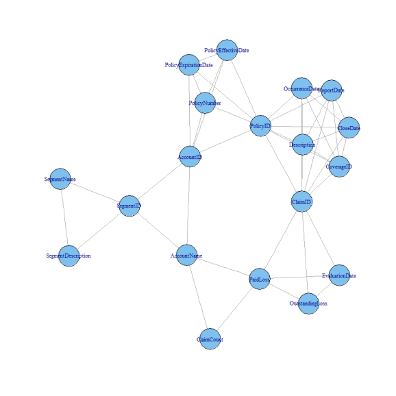
I love this. Somehow the account name, but not the account ID is related to claim count. Has the query been properly designed? Policy information sits by itself, walled off from the marketing segment and the claims information, as it should be. There are just two steps from paid loss to business segment. This also makes a bit of sense.
There are several dozen things that I'd like to do with this, but they'll have to wait until tomorrow or later. I'm going to keep playing with this as I think it's a fantastic way to get an initial read on the complexity of a new database. There are several things in this world that I absolutely love. One of them is a map. Another? Metadata!
sessionInfo()

## R version 3.0.2 (2013-09-25)
## Platform: x86_64-w64-mingw32/x64 (64-bit)
##
## locale:
## [1] LC_COLLATE=English_United States.1252
## [2] LC_CTYPE=English_United States.1252
## [3] LC_MONETARY=English_United States.1252
## [4] LC_NUMERIC=C
## [5] LC_TIME=English_United States.1252
##
## attached base packages:
## [1] stats     graphics  grDevices utils     datasets  methods   base
##
## other attached packages:
## [1] knitr_1.4.1      RWordPress_0.2-3 igraph_0.6.6     RODBC_1.3-8
##
## loaded via a namespace (and not attached):
## [1] digest_0.6.3   evaluate_0.4.7 formatR_0.9    RCurl_1.95-4.1
## [5] stringr_0.6.2  tools_3.0.2    XML_3.98-1.1   XMLRPC_0.3-0
