It is well known, though often dismissed, that the areas of spatial units (cells, pixels) based on unprojected coordinates (longitude-latitude degrees, arc-minutes or arc-seconds) are wildly inconsistent across the globe. Towards the poles, as the longitude meridians approach each other, the actual ground width of the pixels sharply decreases. So, for non-tropical regions, the actual area covered by these pixels can be quite far from the nominal “approximately 1 km at the Equator” (or 10 km, etc.) which is often referred in biogeography and macroecology studies.

The function below combines several tools from the ‘terra’ R package to compute the (mean or centroid) pixel area for a given unprojected raster map. By default, it also produces a map illustrating the latitudinal variation in the pixel areas.

pixelArea <- function(r, # SpatRaster
                       type = "mean", # can also be "centroid"
                       unit = "m",  # can also be "km"
                       mask = TRUE,  # to consider only areas of non-NA pixels
                       map = TRUE) {
  # version 1.2 (23 Jan 2024)
  
  stopifnot(inherits(r, "SpatRaster"),
            type %in% c("mean", "centroid"))
  
  r_size <- terra::cellSize(r, unit = unit, mask = mask)
  if (map) terra::plot(r_size, main = paste0("Pixel area (", unit, "2)"))
  areas <- terra::values(r_size, mat = FALSE, dataframe = FALSE, na.rm = FALSE)  # na.rm must be FALSE for areas[centr_pix] to be correct
  
  if (type == "mean") {
    cat(paste0("Mean pixel area (", unit, "2):\n"))
    return(mean(areas, na.rm = TRUE))
  }
  
  if (type == "centroid") {
    r_pol <- terra::as.polygons(r * 0, aggregate = TRUE)
    centr <- terra::centroids(r_pol)
    if (map) {
      if (!mask) terra::plot(r_pol, lwd = 0.2, add = TRUE)
      terra::plot(centr, pch = 4, col = "blue", add = TRUE)
    }
    
    centr_pix <- terra::cellFromXY(r, terra::crds(centr))
    cat(paste0("Centroid pixel area (", unit, "2):\n"))
    return(areas[centr_pix])
  }
}

Here’s a usage example for a central European country:

elev_switz <- geodata::elevation_30s("Switzerland", path = tempdir())
terra::plot(elev_switz)

terra::res(elev_switz)
# 0.008333333 degree resolution
# i.e. half arc-minute, or 30 arc-seconds (1/60/2)
# "approx. 1 km at the Equator"

pixelArea(elev_switz, unit = "km")
# Mean pixel area (km2):
# [1] 0.5892033

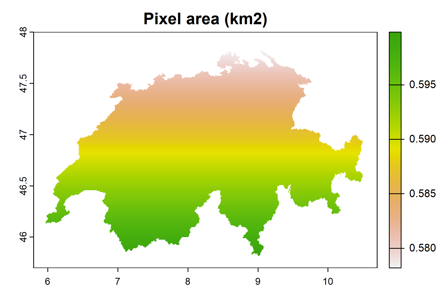
As you can see, pixel area here is quite different from 1 squared km, and Switzerland isn’t even one of the northernmost countries. So, when using unprojected rasters (e.g. WorldClim, CHELSA climate, Bio-ORACLE, MARSPEC and so many others) in your analysis, consider choosing the spatial resolution that most closely matches the resolution that you want in your study region, rather than the resolution at the Equator when this is actually far away. This was done e.g. in this paper (see Supplementary Files – ExtendedMethods.docx).

You can read more details about geographic areas in the help file of the terra::expanse() function. Feedback welcome!