Hello, hope you have your Yorkshire tea ready this is going to be a new series on the blog in which each month I am going to be tackling Kaggles monthly playground series. Find the link to Januarys below feel free

https://www.kaggle.com/competitions/playground-series-s3e1

So let’s get started

EDA

Above is the structure of the training dataset. The target variable is the MedHouseVal and the other variables can be used as features in the model apart from ID which is just an identification column. Latitude and Longitude probably wouldn’t be good to just put into the mode as lots of different values could cause delays in training or it might not be that informative. Generally, areas have higher prices so let’s check that.

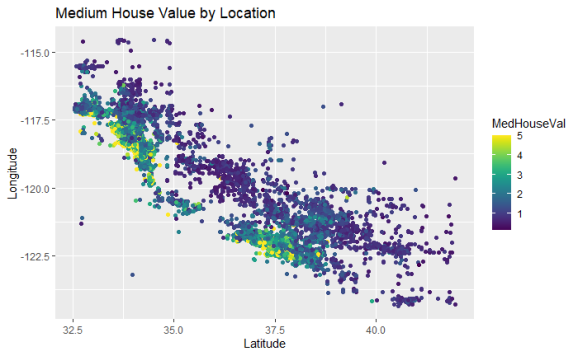
The highest medium house value areas are grouped together. They must be in San Francisco and Los Angeles and they are generally closer to the coast. I’m going to investigate using K Means clustering to give the model this information about the location.

Overall it looks like Medium income is the most correlated to the target variable. This is obvious because more earnings mean you spend more money on a bigger nicer house. There looks to be absolutely no correlation with house age which also makes sense as all sorts of houses are built all the time.

K Means Clustering

locs_test = test_fin %>% select(Latitude, Longitude)


all_locs = locs_test %>% bind_rows(locs)

# creating the kmeans clustering for a range a values of K
clusters <- 
  tibble(k = 1:100) %>% #setting a range of k values 
  mutate(
    kclust = map(k, ~kmeans(all_locs, .x)), #using the kmeans function to run kmeans with different value of k
    tidied = map(kclust, tidy),
    glanced = map(kclust, glance),
    augmented = map(kclust, augment, all_locs)
  )


# function to test the how model accuracy is impacted by k value chosen 

kmeans_test = function(x) {
assing2 =  clusters %>% 
  unnest(cols = c(augmented)) %>%
       filter(k == x) %>% 
             select(Latitude, Longitude, .cluster)  %>%
          distinct() %>% 
                left_join(train, by = c("Latitude", "Longitude")) %>% 
                    select(.cluster, MedInc, MedHouseVal)
 
lm_mod = lm(MedHouseVal ~., assing2)


fin = tibble(summary(lm_mod)$adj.r.squared) %>% 
                    mutate(k = x)

colnames(fin)[1] = "rsqr"
    
return(fin)
    
    }


ks = 2:99

fin_frame = map_dfr(ks, kmeans_test)

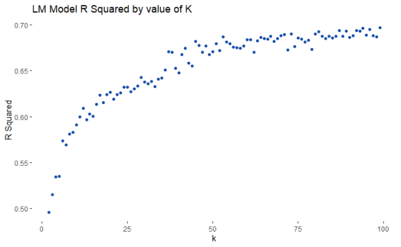
In order to test the use of k means clustering on the model I ran k means for a range of k values and then fitted a simple regression model on each value of k. The point here is to create clusters most informative for the final model, therefore, I plotted the r squared value for each value of K, as a result, the graph shows how the number of clusters impacts model performance. The more clusters the better the model performed therefore for the final model I set the number of clusters to 99.

Model Training

#selecting the features for the model 
train2 = train %>% left_join(assignments, by = c("Latitude", "Longitude")) %>%
                        select(MedInc, AveRooms, AveBedrms, Population, AveOccup, MedHouseVal, .cluster)

#using rsample to create train and test split 
split = initial_split(train2, prop = 0.75, strata = MedHouseVal)


train_data = training(split)
test_data = testing(split)



## creating the folds to tune the model 
set.seed(234)
cali_folds <- vfold_cv(train_data, strata = MedHouseVal)
cali_folds



ranger_recipe <- 
  recipe(formula = MedHouseVal ~ ., data = train_data) 

ranger_spec <- 
  rand_forest(mtry = tune(), min_n = tune(), trees = 1000) %>% 
  set_mode("regression") %>% 
  set_engine("ranger") 

ranger_workflow <- 
  workflow() %>% 
  add_recipe(ranger_recipe) %>% 
  add_model(ranger_spec) 

doParallel::registerDoParallel()

set.seed(6815)
ranger_tune <-
  tune_grid(ranger_workflow, resamples = cali_folds, grid = 5)

I used the use models package to generate the code needed in order to train this first random forest model. The final random forest model had an RMSE of 0.63 which is a good baseline but there are other model frameworks to try to see if this can be improved. The first model framework tried was XG Boost

xgboost_recipe <- 
  recipe(formula = MedHouseVal ~ ., data = train_data) %>% 
  step_novel(all_nominal_predictors()) %>% 
  step_dummy(all_nominal_predictors(), one_hot = TRUE) %>% 
  step_zv(all_predictors()) 


xgb_spec <-
  boost_tree(
    trees = tune(),
    mtry = tune(),
    min_n = tune(),
    learn_rate = 0.01
  ) %>%
  set_engine("xgboost") %>%
  set_mode("regression")

xgb_wf <- workflow(xgboost_recipe, xgb_spec)
xgb_wf



library(finetune)
doParallel::registerDoParallel()

set.seed(234)
xgb_game_rs <-
  tune_race_anova(
    xgb_wf,
    cali_folds,
    grid = 20,
    control = control_race(verbose_elim = TRUE)
  )


plot_race(xgb_game_rs)

Moving on to an xgboost model in order to tune the model I used the tune race function from the tidymodels packages. This speeds up the tuning process as parameters for the model which do not lead to an accurate model are eliminated and the most accurate model is the one that is left in the end.

I took the best-performing model and fitted a xgboost model with those parameters. Finally, I decided to investigate a light gbm model which I have never done before but is a popular model to do well on Kaggle.

light_model<-
parsnip::boost_tree(
mode = "regression",
trees = 1000,
min_n = tune(),
learn_rate = tune(),
tree_depth = tune()
) %>%
set_engine("lightgbm", objective = "rmse",verbose=-1)


light_workflow <- 
  workflow() %>% 
  add_recipe(ranger_recipe) %>% 
  add_model(light_model) 

doParallel::registerDoParallel()

set.seed(6815)
light_tune <-
  tune_grid(light_workflow, resamples = cali_folds, grid = 50)

I first trained a model to get an idea of the optimum parameter values as seen from the code above and then produced a final model and tested it on the testing data.

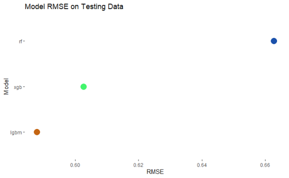
The lightgbm model is the most accurate in the comparison. However, I still think the other models can be used to aid in an accurate prediction for the final testing data. Therefore I am going to use prediction from all models but I will weight it by whichever leaves the most accurate prediction.

I tested the weightings for 0 to 100 for each of the 3 models to see which model would be the most accurate. Above is the top 10 weightings and it is dominated by heavy weighting to the lgbm model. Therefore this is the lighting that will be used for my final entry into the competition.

Final Result

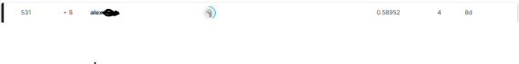
This was my final position it was 531st out of 690. Therefore I wasn’t particularly close to the top entrants. One mistake I made is when doing the final model I didn’t retrain it on the full training dataset. I don’t think this is the reason I didn’t win but might have made some difference to the final result.

References

https://www.r-bloggers.com/2020/08/how-to-use-lightgbm-with-tidymodels/

https://juliasilge.com/blog/shelter-animals/