Summary

In this tutorial participants will learn about biological data analysis with R and Unix/Linux tools. We begin with an introduction to bioinformatics and omics data analysis, and conclude with the walkthrough of a simple bioinformatics workflow for aligning transcriptomic sequences with genomic data.

Questions

• What is bioinformatics?
• What data we will be working with?
• What are some databases that I can use to collect omics data?
• What are common file formats for transcriptomic and genomic data?
• How can different types of omics data be used together?

Objectives

• Learn about key aspects of the bioinformatics field.
• Become familiar with how transcriptomic and genomic data is structured.
• Learn BASH programming skills for collecting omics data.
• Be able to use bioinformatics software tools to prepare omics data for analysis.

What is Bioinformatics?

Bioinformatics is an interdisciplinary field that combines techniques and knowledge from both computer science and biology. It is a computational field that involves the analysis of complex omics data. This commonly includes DNA, RNA, or protein sequence data.

Bioinformatics data is generated through various omics technologies used to analyze different types of biological molecules. Biological data produced by omics technologies include:

• genomic
• transcriptomic
• proteomic
• metabolomic

Bioinformaticians use computer programming to investigate the patterns in omics data. Furthermore, different types of omics data can be combined to find complex and subtle relationships.

The following are some well known online omics databases.

• Database of Genomic Structural Variation (dbVar) – archives insertions, deletions, duplications, inversions, mobile element insertions, translocations, and complex chromosomal rearrangements
• Database of Genotypes and Phenotypes (dbGaP) – developed to archive and distribute the data and results from studies that have investigated the interaction of genotype and phenotype in Humans
• Database of Single Nucleotide Polymorphisms (dbSNP) – archives multiple small-scale variations that include insertions/deletions, microsatellites, and non-polymorphic variants
• GenBank – the NIH genetic sequence database, which is an annotated collection of all publicly available DNA sequences
• The Reference Sequences (RefSeq) collection – provides a comprehensive, integrated, non-redundant, well-annotated set of sequences, including genomic DNA, transcripts, and proteins
• Gene Expression Omnibus (GEO) – a public functional genomics data repository supporting MIAME-compliant data submissions
• Gene Expression Omnibus Datasets (GEO DataSets) – stores curated gene expression DataSets, as well as original Series and Platform records in the Gene Expression Omnibus (GEO) repository
• Genome Data Viewer (GDV) – a genome browser supporting the exploration and analysis of more than 380 eukaryotic RefSeq genome assemblies
• International Genome Sample Resource (IGSR) – from the 1000 Genomes Project that ran between 2008 and 2015, which created the largest public catalogue of human variation and genotype data

Bioinformatics Workflows

A typical bioinformatics or biostatistics data analysis workflow will have multiple steps that may include:

1. experimental design
2. data collection
3. quality control
4. data preparation
5. statistical analysis
6. data visualization
7. interpretation of results

The following graphic depicts a typical workflow for preparing, analyzing, and visualizing results from transcriptomic RNA sequencing data.

In this lesson you will gain experience in performing omics data analysis by working through part of a bioinformatics pipeline for analyzing gene expression data. The steps in the bioinformatics workflow that we will cover in this lesson are:

1. data collection – SRA toolkit
2. quality control – fastqc
3. genomic data format conversion – gffread
4. transcriptomic data alignment – hisat2
5. quantify transcript alignments – featureCounts

A great benefit of developing a common bioinformatics workflow is the ability to create a pipeline, in which the necessary outputs from the previous steps are passed on as inputs to subsequent steps.

The Data Set

As a first step, we will begin with collecting some data for analysis. In this lesson we will be using data from a study of the effects of ultraviolet (UV) radiation on the larvae of the red flour beetle titled “Digital gene expression profiling in larvae of Tribolium castaneum at different periods post UV-B exposure“.

UV radiation is common to many environments and it varies widely in its intensity and composition, such as differing ratios of UV-A and UV-B radiation. The different forms of UV radiation have distinct, and frequently harmful effects on organisms and biological systems.

For example, the following diagram depicts the effects of different forms of UV radiation on skin.

UV radiation is considered an important environmental stressor that organisms need to defend against. There are three primary methods for defending against UV radiation:

• Avoidance
• Photoprotection
• Repair

Since the red flour beetle (Tribolium castaneum) spends much of its life cycle in infested grains, the larvae does not typically experience high levels of UVR. Furthermore, the larvae of the red flour beetle is light in pigmentation and does not appear to employ photoprotective pigments (e.g., melanin) to defend against harmful levels of UV radiation (UVR).

So, how do red flour beetle larvae respond to UVR exposure?

Study Design & Bioinformatics Workflow

In their study, the authors investigated the defense strategy against UV-B radiation in red flour beetle larvae. The following graphical abstract illustrates how the transcriptomic (expression) data was generated, as well as the bioinformatics workflow of the authors.

The following steps were performed by the authors in their bioinformatics analysis, which is described in the “2.4. Bioinformatic analysis” section of the paper:

1. Reads mapping to the reference genome – TopHat
2. Quantification of gene expression level and differential expression analysis – RSEM & DESeq2
3. Gene ontology and Kyoto encyclopedia of genes and genomes pathway enrichment analysis of differentially expressed genes – GOseq & KOBAS
4. Validation by qRT-PCR

So we will be performing similar analysis to the first two parts of the above bioinformatics workflow from the red flour beetle paper. Recall the bioinformatics workflow we will be completing in this tutorial:

1. data collection – SRA toolkit
2. quality control – fastqc
3. genomic data format conversion – gffread
4. transcriptomic data alignment (mapping) – hisat2
5. quantify transcript alignments – featureCounts

Note that we will be using several different types of omics data in our workflow. Remember that data generated by omics technologies include genetic, transcriptomic, proteomic, and metabolomic data.

What is Gene Transcription?

Transcription is the first step in gene expression that involves copying the DNA sequence of a gene to make a RNA molecule. For a protein-coding gene, the RNA copy (transcript) carries the information needed to build a polypeptide (protein or protein subunit).

The transcription of genes can be measured using next-generation sequencing techniques that are able to produce millions of sequences (reads) in a short time. This process is depicted in the following schematic representation of a RNA sequencing protocol.

Transcription can provide genome-wide RNA expression profiles, and is useful for identifying key factors influencing transcription in different environmental conditions.

The Genomic Data

The genomic data we need for the Tribolium castaneum (red flour beetle) can be collected from InsectBase. The red flour beetle is an arthropod in the order Coleoptera and family Tenebrionidae.

Navigate to the Tribolium castaneum organism page of the InsectBase website and under the “Download” section of the page:

• click the red word Genome to begin downloading the reference genome file (e.g., Tribolium_castaneum.genome.fa)
• click the blue word GFF3 to begin downloading the general features file (e.g., Tribolium_castaneum.gff3)

Notice that we are using genomic data from InsectBase instead of BeetleBase, since BeetleBase is no longer available.

Reference Genome

The reference genome we downloaded is in the FASTA file format, and has the .fa file extension. This format is commonly used when storing DNA sequence data.

Note that sequences are expected to be represented in the standard IUB/IUPAC amino acid and nucleic acid codes, with some exceptions.

General Features

The general features file (GFF) is in the GFF3 file structure and has the .gff3 file extension. This format is a tab-delimited text file that is used to describe information about features of a nucleic acid or protein sequence.

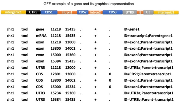
The features of the GFF may include anything from coding sequences (CDS), microRNAs, binding domains, open reading frames (ORFs), etc.

Features Data Conversion

The general features file that we downloaded from InsectBase for Tribolium castaneum is in the gff3 format, but it needs to be in gtf format to use with HISAT2 downstream. Note that there are some important formatting differences between the two general feature file types.

Let’s install and use the gffread command line tool to convert the general features file named Tribolium_castaneum.gff3 from gff3 to gtf format. Check out the manual page for gffread to learn more about the different options (flags).

gffread -E -F -T Tribolium_castaneum.gff3 -o Tribolium.gtf

Notice that the o flag is used to specify the output file name. In the above example Tribolium.gtf is the name of the output gtf file.

The Transcriptomic Data

There are several pieces of transcriptomic data that we will need to collect before we can proceed with the bioinformatics analysis.

The SRA Toolkit allows you to retrieve data from the sequence read archive (SRA) for a specific research project using the associated accession number.

After installing the SRA Toolkit, we can proceed with collecting the transcriptomic data we need for our bioinformatics analysis. Remember that we are using the transcriptomic data described in the “Digital gene expression profiling in larvae of Tribolium castaneum at different periods post UV-B exposure” paper.

First, let’s search the paper for “accession” (Mac: command+f, Windows: ctrl+f) and copy the Accession No (e.g., PRJNA504739).

We’ll use the SRA Run Selector to find the list of sequencing read accession numbers for the set of transcriptomic data associated with the study accession number (e.g., PRJNA504739) like shown below.

Retrieve the SRA accession numbers for all of the samples associated with the study by selecting to download the total accession list from the “Select” section of the resulting page.

Now we can download all of the transcriptomic sequence data for the study using the sample accession numbers and SRA toolkit prefetch and fastq-dump commands in the shell (e.g., BASH or Zsh). Make sure to use the gzip flag to compress the files as they are downloaded.

prefetch SRR8288561 SRR8288562 SRR8288563 SRR8288564 SRR8288557 SRR8288560 SRR8288558 SRR8288559 SRR8288565 SRR8288566 SRR8288567 SRR8288568
fastq-dump --gzip SRR8288561
fastq-dump --gzip SRR8288562
fastq-dump --gzip SRR8288563
fastq-dump --gzip SRR8288564
fastq-dump --gzip SRR8288557
fastq-dump --gzip SRR8288560
fastq-dump --gzip SRR8288558
fastq-dump --gzip SRR8288559
fastq-dump --gzip SRR8288565
fastq-dump --gzip SRR8288566
fastq-dump --gzip SRR8288567
fastq-dump --gzip SRR8288568

It is possible to combine lines of shell code using the semicolon ; operator as follows.

prefetch SRR8288561 SRR8288562 SRR8288563 SRR8288564 SRR8288557 SRR8288560 SRR8288558 SRR8288559 SRR8288565 SRR8288566 SRR8288567 SRR8288568
fastq-dump --gzip SRR8288561; fastq-dump --gzip SRR8288562; fastq-dump --gzip SRR8288563; fastq-dump --gzip SRR8288564; fastq-dump --gzip SRR8288557; fastq-dump --gzip SRR8288560
fastq-dump --gzip SRR8288558; fastq-dump --gzip SRR8288559; fastq-dump --gzip SRR8288565; fastq-dump --gzip SRR8288566; fastq-dump --gzip SRR8288567; fastq-dump --gzip SRR8288568

Note that if a shell command is taking a long time to run in the terminal, you may use the ctrl+c keyboard shortcut to kill it and force it to stop running.

Transcription Sequences

In this workshop we will be using transcription sequence data in the FASTQ format. Each sequence in the file typically has the following four lines of information.

• A line beginning with @ followed by a sequence identifier and optional description (comment)
• The raw sequence letters
• A line beginning with + and sometimes followed by the same comment as the first line
• A line encoding the quality values for the sequence in line 2 and with the same numbers of symbols as letters in the sequence

Quality Control

An important part of any bioinformatics analysis workflow is the assessment and quality control (QC) of your data. In this lesson we are using RNA sequencing reads, which may need to be cleaned if they are raw and include extra pieces of unnecessary data (e.g., adapter sequences).

To check if the transcriptomic data that we downloaded needs to be trimmed and cleaned up, we will install the FastQC bioinformatics software tool.

Let’s use the following fastqc command in the shell to view the quality of one of the sequence read data sets. We are using the extract option (flag) to decompress and extract the zipped output files.

fastqc SRR8288560.fastq.gz --extract

Now we can check the results that we received from the analysis of this sample to look for some common quality issues with RNA sequencing (RNA-Seq) data.

In the above report there is one failed metric of “per base sequence content”, which is indicated by the red x. This is not an issue for our data since most RNA-Seq library preparation protocols result in a clear non-uniform distribution of the first 10-15 bases.

There is also a warning given for the “sequence duplication levels” metric, indicated by the orange exclamation in the report below.

Again, this is expected for RNA-seq data and is not an issue since duplicate reads will be observed for highly abundant transcripts.

Sequence Alignment

Next, we need to prepare the transcriptomic sequence data files for statistical analysis by aligning (mapping) the reads to the reference genome. This is an important part of our bioinformatics analysis workflow and involves mapping the shattered (fragmented) reads to a reference genome.

Let’s use the HISAT2 command line tool to map the transcriptomic sequence reads to the reference genome of Tribolium castaneum. Make sure to first install the tool and check out the manual page for HISAT2 to learn more about the different options (flags).

Note that we are using HISAT2 rather than TopHat2, since TopHat2 is no longer supported and has been replaced with HISAT2.

First, we need to use the hisat2-build command to build a HISAT2 index from the set of nucleotide sequences for Tribolium castaneum contained in the reference genome fasta file (e.g., Tribolium_castaneum.genome.fa).

hisat2-build Tribolium_castaneum.genome.fa TriboliumBuild

Now we can use the hisat2 command to map the RNA sequencing reads (transcripts) for each sample to the reference genome as follows.

hisat2 -q -x TriboliumBuild -U SRR8288561.fastq.gz -S SRR8288561_accepted_hits.sam
hisat2 -q -x TriboliumBuild -U SRR8288562.fastq.gz -S SRR8288562_accepted_hits.sam
hisat2 -q -x TriboliumBuild -U SRR8288563.fastq.gz -S SRR8288563_accepted_hits.sam
hisat2 -q -x TriboliumBuild -U SRR8288564.fastq.gz -S SRR8288564_accepted_hits.sam 
hisat2 -q -x TriboliumBuild -U SRR8288557.fastq.gz -S SRR8288557_accepted_hits.sam
hisat2 -q -x TriboliumBuild -U SRR8288560.fastq.gz -S SRR8288560_accepted_hits.sam
hisat2 -q -x TriboliumBuild -U SRR8288558.fastq.gz -S SRR8288560_accepted_hits.sam
hisat2 -q -x TriboliumBuild -U SRR8288567.fastq.gz -S SRR8288560_accepted_hits.sam
hisat2 -q -x TriboliumBuild -U SRR8288568.fastq.gz -S SRR8288560_accepted_hits.sam
hisat2 -q -x TriboliumBuild -U SRR8288559.fastq.gz -S SRR8288560_accepted_hits.sam
hisat2 -q -x TriboliumBuild -U SRR8288565.fastq.gz -S SRR8288560_accepted_hits.sam
hisat2 -q -x TriboliumBuild -U SRR8288566.fastq.gz -S SRR8288560_accepted_hits.sam

Notice that the S flag is used to specify the output file name for each sample, which ends in the .sam extension.

Sequence Alignment Maps

The sequence alignment files we generated for each sample are stored in the sequence alignment/map (SAM) format and have the .sam file extension. SAM files are in a TAB-delimited text format with an optional header section and an alignment section.

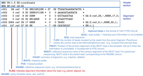
As we can see above, the alignment section has multiple fields that are used to describe each aligned sequence.

Transcript Quantification

Now that we have the transcript sequence reads aligned to the reference genome, we can quantify (count) the number of sequencing read fragments that map (align) to each general feature from the features file.

Let’s use the featureCounts function of the Rsubread library to count the number of transcripts that map to each feature in the Tribolum castaneum reference genome. The ? operator can be prepended to a function name (e.g., ?featurecounts) in R to retrieve more information about the function.

Note that we are using featureCounts instead of RSEM, since featureCounts is efficient and has a low run time.

To make the next steps more simple, set your working directory in R as follows.

setwd("/YOUR/DIRECTORY/PATH")

Next make sure to install the BiocManager package, if you do not already have it installed.

install.packages("BiocManager")

Then you can use BiocManager to install the Rsubread package, if you do not already have it installed.

if (!require("BiocManager", quietly = TRUE))
  install.packages("BiocManager")
BiocManager::install("Rsubread")

Remember to load the Rsubread library before you attempt to use the featureCounts function.

library(Rsubread)

Now to quantify the read fragments that map to the features of the red flour beetle genome, we will use the fetureCounts function in R with each of the sample sam files and the general features file.

# control samples at 4h
cntrl1_fc_4h <- featureCounts(files="SRR8288561_accepted_hits.sam", annot.ext="Tribolium.gtf", isGTFAnnotationFile=TRUE)
cntrl2_fc_4h <- featureCounts(files="SRR8288562_accepted_hits.sam", annot.ext="Tribolium.gtf", isGTFAnnotationFile=TRUE)
cntrl3_fc_4h <- featureCounts(files="SRR8288563_accepted_hits.sam", annot.ext="Tribolium.gtf", isGTFAnnotationFile=TRUE)
# control samples 24h
cntrl1_fc_24h <- featureCounts(files="SRR8288558_accepted_hits.sam", annot.ext="Tribolium.gtf", isGTFAnnotationFile=TRUE)
cntrl2_fc_24h <- featureCounts(files="SRR8288567_accepted_hits.sam", annot.ext="Tribolium.gtf", isGTFAnnotationFile=TRUE)
cntrl3_fc_24h <- featureCounts(files="SRR8288568_accepted_hits.sam", annot.ext="Tribolium.gtf", isGTFAnnotationFile=TRUE)
# treatment samples at 4h
treat1_fc_4h <- featureCounts(files="SRR8288564_accepted_hits.sam", annot.ext="Tribolium.gtf", isGTFAnnotationFile=TRUE)
treat2_fc_4h <- featureCounts(files="SRR8288557_accepted_hits.sam", annot.ext="Tribolium.gtf", isGTFAnnotationFile=TRUE)
treat3_fc_4h <- featureCounts(files="SRR8288560_accepted_hits.sam", annot.ext="Tribolium.gtf", isGTFAnnotationFile=TRUE)
# treatment samples 24h
treat1_fc_24h <- featureCounts(files="SRR8288559_accepted_hits.sam", annot.ext="Tribolium.gtf", isGTFAnnotationFile=TRUE)
treat2_fc_24h <- featureCounts(files="SRR8288565_accepted_hits.sam", annot.ext="Tribolium.gtf", isGTFAnnotationFile=TRUE)
treat3_fc_24h <- featureCounts(files="SRR8288566_accepted_hits.sam", annot.ext="Tribolium.gtf", isGTFAnnotationFile=TRUE)

Notice that with each use of the featureCounts command the sam file is specified using the files argument. The general features file (e.g., Tribolium.gtf) is specified with the annot.ext argument. Additionally, we need to set isGTFAnnotationFile equal to TRUE since we are using a gtf formatted general features file.

Before we can move on to any statistical analysis, we need to prepare the data by combining (merging) all of the results for each quantified sam file to a single data frame. Note that data frames in R are used to store two-dimensional (2D) data.

tribolium_counts <- data.frame(
  SRR8288561 = unname(cntrl1_fc_4h$counts),
  SRR8288562 = unname(cntrl2_fc_4h$counts),
  SRR8288563 = unname(cntrl3_fc_4h$counts),
  SRR8288558 = unname(cntrl1_fc_24h$counts),
  SRR8288567 = unname(cntrl2_fc_24h$counts),
  SRR8288568 = unname(cntrl3_fc_24h$counts),
  SRR8288564 = unname(treat1_fc_4h$counts),
  SRR8288557 = unname(treat2_fc_4h$counts),
  SRR8288560 = unname(treat3_fc_4h$counts),
  SRR8288559 = unname(treat1_fc_24h$counts),
  SRR8288565 = unname(treat2_fc_24h$counts),
  SRR8288566 = unname(treat3_fc_24h$counts)
)

Next, let’s take a look at what the first few lines (top) of the merged counts data frame looks like.

head(tribolium_counts)

We can see that the gene names are not assigned to each row of the data frame at this point. So we’ll set the row names of the merged counts data frame using the row names from a data frame for one of the samples as follows.

rownames(tribolium_counts) <- rownames(cntrl1_fc_4h$counts)

To verify that the merged counts data frame was properly updated, let’s see what the top of the data frame looks like.

head(tribolium_counts)

As a final step, let’s store (save) the merged gene counts in a csv file named triboliumCounts.csv using the write.csv function.

write.csv(tribolium_counts, "triboliumCounts.csv")

The merged gene count data is now saved and in a format we can use for downstream biostatistical analysis, such as differential expression (DE) analysis.

Key Points & Tips

• Different types of omics data are often combined in bioinformatics workflows
• Explore available omics databases before you design your analysis workflow
• Determine the order of input and output files for each step of your workflow
• Investigate the supplemental materials of research study papers
• Make sure to install any necessary software in advance
• Carefully name and store your raw and calculated data files

Code & Data

A shell script with the code for each of the omics data collection and preparation steps is provided on my GitHub -> here <-

A R script with the code for quantifying the transcriptomic data is provided -> here <-

The comma separated variable (CSV) file named triboliumCounts.csv with the final merged gene count results can be found -> here <-