Player Performance Estimation using AI Collaborative Filtering

Posted on May 15, 2022 by Tinniam V Ganesh in R bloggers | 0 Comments

[This article was first published on R – Giga thoughts …, and kindly contributed to R-bloggers]. (You can report issue about the content on this page here)

Want to share your content on R-bloggers? click here if you have a blog, or here if you don't.

1. Introduction

Often times before crucial matches, or in general, we would like to know the performance of a batsman against a bowler or vice-versa, but we may not have the data. We generally have data where different batsmen would have faced different sets of bowlers with certain performance data like ballsFaced, totalRuns, fours, sixes, strike rate and timesOut. Similarly different bowlers would have performance figures(deliveries, runsConceded, economyRate and wicketTaken) against different sets of batsmen. We will never have the data for all batsmen against all bowlers. However, it would be good estimate the performance of batsmen against a bowler, even though we do not have the performance data. This could be done using collaborative filtering which identifies and computes based on the similarity between batsmen vs bowlers & bowlers vs batsmen.

This post shows an approach whereby we can estimate a batsman’s performance against bowlers even though the batsman may not have faced those bowlers, based on his/her performance against other bowlers. It also estimates the performance of bowlers against batsmen using the same approach. This is based on the recommender algorithm which is used to recommend products to customers based on their rating on other products.

This idea came to me while generating the performance of batsmen vs bowlers & vice-versa for 2 IPL teams in this IPL 2022 with my Shiny app GooglyPlusPlus. I found that there were some batsmen for which there was no data against certain bowlers, probably because they are playing for the first time in their team or because they were new. While pondering on this problem, I realized that this problem formulation is similar to the problem formulation for the famous Netflix movie recommendation problem, in which user’s ratings for certain movies are known and based on these ratings, the recommender engine can generate ratings for movies not yet seen.

This post estimates a player’s (batsman/bowler) using the recommender engine This post is based on R package recommenderlab

“Michael Hahsler (2021). recommenderlab: Lab for Developing and Testing Recommender Algorithms. R package version 0.2-7. https://github.com/mhahsler/recommenderlab”

Note 1: Thw data for this analysis is taken from Cricsheet after being processed by my R package yorkr.

You can also read this post in RPubs at Player Performance Estimation using AI Collaborative Filtering

A PDF copy of this post is available at Player Performance Estimation using AI Collaborative Filtering.pdf

You can download this R Markdown file and the associated data and perform the analysis yourself using any other recommender engine from Github at playerPerformanceEstimation

Problem statement

In the table below we see a set of bowlers vs a set of batsmen and the number of times the bowlers got these batsmen out.
By knowing the performance of the bowlers against some of the batsmen we can use collaborative filter to determine the missing values. This is done using the recommender engine.

The Recommender Engine works as follows. Let us say that there are feature vectors $x^1$ , $x^2$ and $x^3$ for the 3 bowlers which identify the characteristics of these bowlers (“fast”, “lateral drift through the air”, “movement off the pitch”). Let each batsman be identified by parameter vectors $\theta^1$ , $\theta^2$ and so on

For e.g. consider the following table

Then by assuming an initial estimate for the parameter vector $\theta$ and the feature vector xx we can formulate this as an optimization problem which tries to minimize the error for $\theta^T*x$ This can work very well as the algorithm can determine features which cannot be captured. So for e.g. some particular bowler may have very impressive figures. This could be due to some aspect of the bowling which cannot be captured by the data for e.g. let’s say the bowler uses the ‘scrambled seam’ when he is most effective, with a slightly different arc to the flight. Though the algorithm cannot identify the feature as we know it, but the ML algorithm should pick up intricacies which cannot be captured in data.

Hence the algorithm can be quite effective.

Note: The recommender lab performance is not very good and the Mean Square Error is quite high. Also, the ROC and AUC curves show that not in aLL cases the algorithm is doing a clean job of separating the True positives (TPR) from the False Positives (FPR)

Note: This is similar to the recommendation problem

The collaborative optimization object can be considered as a minimization of both $\theta$ and the features x and can be written as

J( $x^{(1)},x^{(2)},..x^{(n_{u})}$ , $\theta^{(1)},\theta^{(2)},..,\theta^{(n_{m})}$ }= 1/2 $\sum(\theta^{j})^{T}x^{i}- y^{(i,j)})^{2} + \lambda\sum\sum (x_{k}^{i})^{2} + \lambda\sum\sum (_\theta{k}^{j})^{2}$

The collaborative filtering algorithm can be summarized as follows

Initialize $\theta^1$ , $\theta^2$ … $\theta^{n_{u}}$ and the set of features be $x^1$ , $x^2$ , … , $x^{n_{m}}$ to small random values
Minimize J( $\theta^1$ , $\theta^2$ … $\theta^{n_{u}}$ , $x^1$ , $x^2$ , … , $x^{n_{m}}$ ) using gradient descent. For every
j=1,2, … $n_{u}$ , i= 1,2,.., $n_{m}$
$x_{k}^{i}$ := $x_{k}^{i}$ – $\alpha$ ( $\sigma$ $(\theta^j)^T$ ) $x^i$ – $y^(i,j)\theta_{k}^{j} + \lambda x_{k}^i$

&

$\theta_{k}^{i}$ := $\theta_{k}^{i}$ – $\alpha$ ( $\sigma$ $(\theta^j)^T)x^i - y^(i,j)\theta_{k}^{j} + \lambda x_{k}^i$
Hence for a batsman with parameters $\theta$ and a bowler with (learned) features x, predict the “times out” for the player where the value is not known using $\theta^Tx$

The above derivation for the recommender problem is taken from Machine Learning by Prof Andrew Ng at Coursera from the lecture Collaborative filtering

There are 2 main types of Collaborative Filtering(CF) approaches

User based Collaborative Filtering User-based CF is a memory-based algorithm which tries to mimics word-of-mouth by analyzing rating data from many individuals. The assumption is that users with similar preferences will rate items similarly.
Item based Collaborative Filtering Item-based CF is a model-based approach which produces recommendations based on the relationship between items inferred from the rating matrix. The assumption behind this approach is that users will prefer items that are similar to other items they like.

1a. A note on ROC and Precision-Recall curves

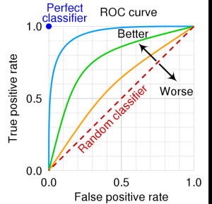
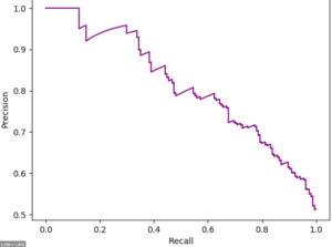
A small note on interpreting ROC & Precision-Recall curves in the post below

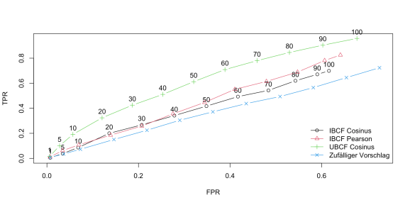
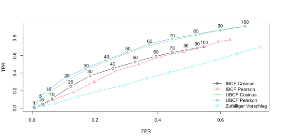
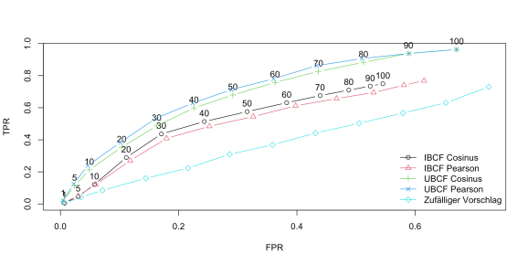
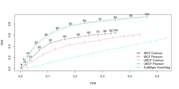
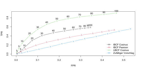
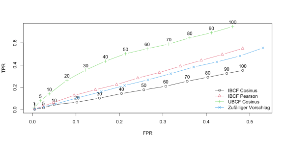
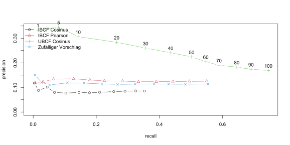
ROC Curve: The ROC curve plots the True Positive Rate (TPR) against the False Positive Rate (FPR). Ideally the TPR should increase faster than the FPR and the AUC (area under the curve) should be close to 1

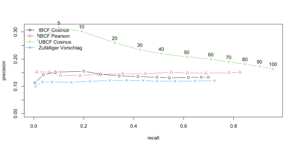
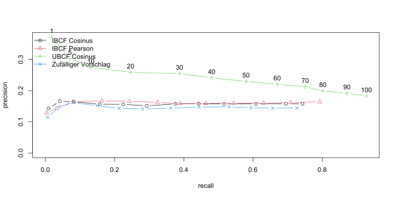
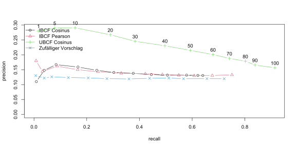
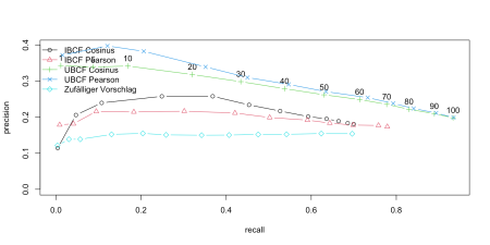
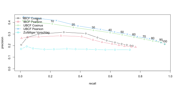
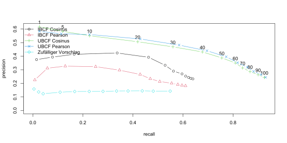
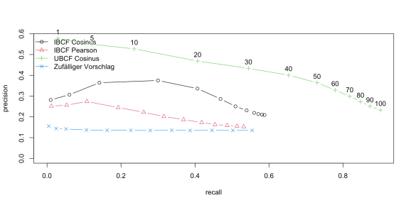
Precision-Recall: The precision-recall curve shows the tradeoff between precision and recall for different threshold. A high area under the curve represents both high recall and high precision, where high precision relates to a low false positive rate, and high recall relates to a low false negative rate

library(reshape2)
library(dplyr)
library(ggplot2)
library(recommenderlab)
library(tidyr)
load("recom_data/batsmenVsBowler20_22.rdata")

2. Define recommender lab helper functions

Helper functions for the RMarkdown notebook are created

eval – Gives details of RMSE, MSE and MAE of ML algorithm
evalRecomMethods – Evaluates different recommender methods and plot the ROC and Precision-Recall curves

# This function returns the error for the chosen algorithm and also predicts the estimates
# for the given data
eval <- function(data, train1, k1,given1,goodRating1,recomType1="UBCF"){
  set.seed(2022)
  e<- evaluationScheme(data,
                       method = "split",
                       train = train1,
                       k = k1,
                       given = given1,
                       goodRating = goodRating1)
  
  r1 <- Recommender(getData(e, "train"), recomType1)
  print(r1)
  
  p1 <- predict(r1, getData(e, "known"), type="ratings")
  print(p1)
  
  error = calcPredictionAccuracy(p1, getData(e, "unknown"))
  
  print(error)
  p2 <- predict(r1, data, type="ratingMatrix")
  p2
}
# This function will evaluate the different recommender algorithms and plot the AUC and ROC curves
evalRecomMethods <- function(data,k1,given1,goodRating1){
  set.seed(2022)
  e<- evaluationScheme(data,
                       method = "cross",
                       k = k1,
                       given = given1,
                       goodRating = goodRating1)
  
  models_to_evaluate <- list(
    `IBCF Cosinus` = list(name = "IBCF", 
                          param = list(method = "cosine")),
    `IBCF Pearson` = list(name = "IBCF", 
                          param = list(method = "pearson")),
    `UBCF Cosinus` = list(name = "UBCF",
                          param = list(method = "cosine")),
    `UBCF Pearson` = list(name = "UBCF",
                          param = list(method = "pearson")),
    `Zufälliger Vorschlag` = list(name = "RANDOM", param=NULL)
  )
  
  n_recommendations <- c(1, 5, seq(10, 100, 10))
  list_results <- evaluate(x = e, 
                           method = models_to_evaluate, 
                           n = n_recommendations)
  plot(list_results, annotate=c(1,3), legend="bottomright")
  plot(list_results, "prec/rec", annotate=3, legend="topleft")
}

3. Batsman performance estimation

The section below regenerates the performance for batsmen based on incomplete data for the different fields in the data frame namely balls faced, fours, sixes, strike rate, times out. The recommender lab allows one to test several different algorithms all at once namely

User based – Cosine similarity method, Pearson similarity
Item based – Cosine similarity method, Pearson similarity
Popular
Random
SVD and a few others

3a. Batting dataframe

head(df)


##   batsman1         bowler1 ballsFaced totalRuns fours sixes  SR timesOut
## 1 A Badoni        A Mishra          0         0     0     0 NaN        0
## 2 A Badoni        A Nortje          0         0     0     0 NaN        0
## 3 A Badoni         A Zampa          0         0     0     0 NaN        0
## 4 A Badoni     Abdul Samad          0         0     0     0 NaN        0
## 5 A Badoni Abhishek Sharma          0         0     0     0 NaN        0
## 6 A Badoni      AD Russell          0         0     0     0 NaN        0

3b Data set and data preparation

For this analysis the data from Cricsheet has been processed using my R package yorkr to obtain the following 2 data sets – batsmenVsBowler – This dataset will contain the performance of the batsmen against the bowler and will capture a) ballsFaced b) totalRuns c) Fours d) Sixes e) SR f) timesOut – bowlerVsBatsmen – This data set will contain the performance of the bowler against the difference batsmen and will include a) deliveries b) runsConceded c) EconomyRate d) wicketsTaken

Obviously many rows/columns will be empty

This is a large data set and hence I have filtered for the period > Jan 2020 and < Dec 2022 which gives 2 datasets a) batsmanVsBowler20_22.rdata b) bowlerVsBatsman20_22.rdata

I also have 2 other datasets of all batsmen and bowlers in these 2 dataset in the files c) all-batsmen20_22.rds d) all-bowlers20_22.rds

You can download the data and this RMarkdown notebook from Github at PlayerPerformanceEstimation

Feel free to download and analyze the data and use any recommendation engine you choose

3c. Exploratory analysis

Initially an exploratory analysis is done on the data

df3 <- select(df, batsman1,bowler1,timesOut)
df6 <- xtabs(timesOut ~ ., df3)
df7 <- as.data.frame.matrix(df6)
df8 <- data.matrix(df7)
df8[df8 == 0] <- NA
print(df8[1:10,1:10])


##                 A Mishra A Nortje A Zampa Abdul Samad Abhishek Sharma
## A Badoni              NA       NA      NA          NA              NA
## A Manohar             NA       NA      NA          NA              NA
## A Nortje              NA       NA      NA          NA              NA
## AB de Villiers        NA        4       3          NA              NA
## Abdul Samad           NA       NA      NA          NA              NA
## Abhishek Sharma       NA       NA      NA          NA              NA
## AD Russell             1       NA      NA          NA              NA
## AF Milne              NA       NA      NA          NA              NA
## AJ Finch              NA       NA      NA          NA               3
## AJ Tye                NA       NA      NA          NA              NA
##                 AD Russell AF Milne AJ Tye AK Markram Akash Deep
## A Badoni                NA       NA     NA         NA         NA
## A Manohar               NA       NA     NA         NA         NA
## A Nortje                NA       NA     NA         NA         NA
## AB de Villiers           3       NA      3         NA         NA
## Abdul Samad             NA       NA     NA         NA         NA
## Abhishek Sharma         NA       NA     NA         NA         NA
## AD Russell              NA       NA      6         NA         NA
## AF Milne                NA       NA     NA         NA         NA
## AJ Finch                NA       NA     NA         NA         NA
## AJ Tye                  NA       NA     NA         NA         NA

The dots below represent data for which there is no performance data. These cells need to be estimated by the algorithm

set.seed(2022)
r <- as(df8,"realRatingMatrix")
getRatingMatrix(r)[1:15,1:15]


## 15 x 15 sparse Matrix of class "dgCMatrix"


##    [[ suppressing 15 column names 'A Mishra', 'A Nortje', 'A Zampa' ... ]]


##                                               
## A Badoni         . . . . . . . . . . . . . . .
## A Manohar        . . . . . . . . . . . . . . .
## A Nortje         . . . . . . . . . . . . . . .
## AB de Villiers   . 4 3 . . 3 . 3 . . . 4 3 . .
## Abdul Samad      . . . . . . . . . . . . . . .
## Abhishek Sharma  . . . . . . . . . . . 1 . . .
## AD Russell       1 . . . . . . 6 . . . 3 3 3 .
## AF Milne         . . . . . . . . . . . . . . .
## AJ Finch         . . . . 3 . . . . . . 1 . . .
## AJ Tye           . . . . . . . . . . . 1 . . .
## AK Markram       . . . 3 . . . . . . . . . . .
## AM Rahane        9 . . . . 3 . 3 . . . 3 3 . .
## Anmolpreet Singh . . . . . . . . . . . . . . .
## Anuj Rawat       . . . . . . . . . . . . . . .
## AR Patel         . . . . . . . 1 . . . . . . .


r0=r[(rowCounts(r) > 10),]
getRatingMatrix(r0)[1:15,1:15]


## 15 x 15 sparse Matrix of class "dgCMatrix"


##    [[ suppressing 15 column names 'A Mishra', 'A Nortje', 'A Zampa' ... ]]


##                                              
## AB de Villiers  . 4 3 . . 3 . 3 . . . 4 3 . .
## Abdul Samad     . . . . . . . . . . . . . . .
## Abhishek Sharma . . . . . . . . . . . 1 . . .
## AD Russell      1 . . . . . . 6 . . . 3 3 3 .
## AJ Finch        . . . . 3 . . . . . . 1 . . .
## AM Rahane       9 . . . . 3 . 3 . . . 3 3 . .
## AR Patel        . . . . . . . 1 . . . . . . .
## AT Rayudu       2 . . . . . 1 . . . . 3 . . .
## B Kumar         3 . 3 . . . . . . . . . . 3 .
## BA Stokes       . . . . . . 3 4 . . . 3 . . .
## CA Lynn         . . . . . . . 9 . . . 3 . . .
## CH Gayle        . . . . . 6 . 3 . . . 6 . . .
## CH Morris       . 3 . . . . . . . . . 3 . . .
## D Padikkal      . 4 . . . 3 . . . . . . 3 . .
## DA Miller       . . . . . 3 . . . . . 3 . . .


# Get the summary of the data
summary(getRatings(r0))


##    Min. 1st Qu.  Median    Mean 3rd Qu.    Max. 
##   1.000   3.000   3.000   3.463   4.000  21.000


# Normalize the data
r0_m <- normalize(r0)
getRatingMatrix(r0_m)[1:15,1:15]


## 15 x 15 sparse Matrix of class "dgCMatrix"


##    [[ suppressing 15 column names 'A Mishra', 'A Nortje', 'A Zampa' ... ]]


##                                                                       
## AB de Villiers   .         -0.7857143 -1.7857143 .  .       -1.7857143
## Abdul Samad      .          .          .         .  .        .        
## Abhishek Sharma  .          .          .         .  .        .        
## AD Russell      -2.6562500  .          .         .  .        .        
## AJ Finch         .          .          .         . -0.03125  .        
## AM Rahane        4.6041667  .          .         .  .       -1.3958333
## AR Patel         .          .          .         .  .        .        
## AT Rayudu       -2.1363636  .          .         .  .        .        
## B Kumar          0.3636364  .          0.3636364 .  .        .        
## BA Stokes        .          .          .         .  .        .        
## CA Lynn          .          .          .         .  .        .        
## CH Gayle         .          .          .         .  .        1.5476190
## CH Morris        .          0.3500000  .         .  .        .        
## D Padikkal       .          0.6250000  .         .  .       -0.3750000
## DA Miller        .          .          .         .  .       -0.7037037
##                                                                              
## AB de Villiers   .         -1.7857143 . . . -0.7857143 -1.785714  .         .
## Abdul Samad      .          .         . . .  .          .         .         .
## Abhishek Sharma  .          .         . . . -1.6000000  .         .         .
## AD Russell       .          2.3437500 . . . -0.6562500 -0.656250 -0.6562500 .
## AJ Finch         .          .         . . . -2.0312500  .         .         .
## AM Rahane        .         -1.3958333 . . . -1.3958333 -1.395833  .         .
## AR Patel         .         -2.3333333 . . .  .          .         .         .
## AT Rayudu       -3.1363636  .         . . . -1.1363636  .         .         .
## B Kumar          .          .         . . .  .          .         0.3636364 .
## BA Stokes       -0.6086957  0.3913043 . . . -0.6086957  .         .         .
## CA Lynn          .          5.3200000 . . . -0.6800000  .         .         .
## CH Gayle         .         -1.4523810 . . .  1.5476190  .         .         .
## CH Morris        .          .         . . .  0.3500000  .         .         .
## D Padikkal       .          .         . . .  .         -0.375000  .         .
## DA Miller        .          .         . . . -0.7037037  .         .         .

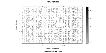
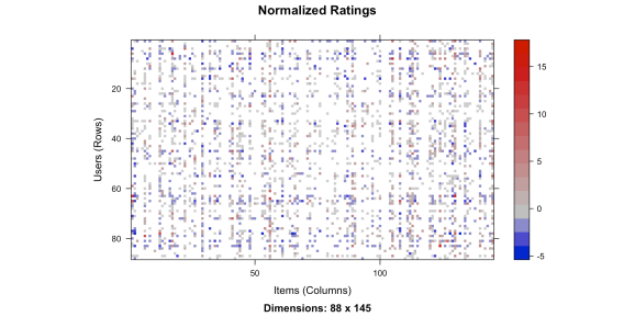
4. Create a visual representation of the rating data before and after the normalization

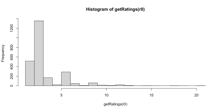
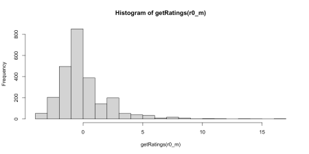
The histograms show the bias in the data is removed after normalization

r0=r[(m=rowCounts(r) > 10),]
getRatingMatrix(r0)[1:15,1:10]


## 15 x 10 sparse Matrix of class "dgCMatrix"


##    [[ suppressing 10 column names 'A Mishra', 'A Nortje', 'A Zampa' ... ]]


##                                    
## AB de Villiers  . 4 3 . . 3 . 3 . .
## Abdul Samad     . . . . . . . . . .
## Abhishek Sharma . . . . . . . . . .
## AD Russell      1 . . . . . . 6 . .
## AJ Finch        . . . . 3 . . . . .
## AM Rahane       9 . . . . 3 . 3 . .
## AR Patel        . . . . . . . 1 . .
## AT Rayudu       2 . . . . . 1 . . .
## B Kumar         3 . 3 . . . . . . .
## BA Stokes       . . . . . . 3 4 . .
## CA Lynn         . . . . . . . 9 . .
## CH Gayle        . . . . . 6 . 3 . .
## CH Morris       . 3 . . . . . . . .
## D Padikkal      . 4 . . . 3 . . . .
## DA Miller       . . . . . 3 . . . .


#Plot ratings
image(r0, main = "Raw Ratings")

#Plot normalized ratings
r0_m <- normalize(r0)
getRatingMatrix(r0_m)[1:15,1:15]


## 15 x 15 sparse Matrix of class "dgCMatrix"


##    [[ suppressing 15 column names 'A Mishra', 'A Nortje', 'A Zampa' ... ]]


##                                                                       
## AB de Villiers   .         -0.7857143 -1.7857143 .  .       -1.7857143
## Abdul Samad      .          .          .         .  .        .        
## Abhishek Sharma  .          .          .         .  .        .        
## AD Russell      -2.6562500  .          .         .  .        .        
## AJ Finch         .          .          .         . -0.03125  .        
## AM Rahane        4.6041667  .          .         .  .       -1.3958333
## AR Patel         .          .          .         .  .        .        
## AT Rayudu       -2.1363636  .          .         .  .        .        
## B Kumar          0.3636364  .          0.3636364 .  .        .        
## BA Stokes        .          .          .         .  .        .        
## CA Lynn          .          .          .         .  .        .        
## CH Gayle         .          .          .         .  .        1.5476190
## CH Morris        .          0.3500000  .         .  .        .        
## D Padikkal       .          0.6250000  .         .  .       -0.3750000
## DA Miller        .          .          .         .  .       -0.7037037
##                                                                              
## AB de Villiers   .         -1.7857143 . . . -0.7857143 -1.785714  .         .
## Abdul Samad      .          .         . . .  .          .         .         .
## Abhishek Sharma  .          .         . . . -1.6000000  .         .         .
## AD Russell       .          2.3437500 . . . -0.6562500 -0.656250 -0.6562500 .
## AJ Finch         .          .         . . . -2.0312500  .         .         .
## AM Rahane        .         -1.3958333 . . . -1.3958333 -1.395833  .         .
## AR Patel         .         -2.3333333 . . .  .          .         .         .
## AT Rayudu       -3.1363636  .         . . . -1.1363636  .         .         .
## B Kumar          .          .         . . .  .          .         0.3636364 .
## BA Stokes       -0.6086957  0.3913043 . . . -0.6086957  .         .         .
## CA Lynn          .          5.3200000 . . . -0.6800000  .         .         .
## CH Gayle         .         -1.4523810 . . .  1.5476190  .         .         .
## CH Morris        .          .         . . .  0.3500000  .         .         .
## D Padikkal       .          .         . . .  .         -0.375000  .         .
## DA Miller        .          .         . . . -0.7037037  .         .         .


image(r0_m, main = "Normalized Ratings")

set.seed(1234)
hist(getRatings(r0), breaks=25)

hist(getRatings(r0_m), breaks=25)

4a. Data for analysis

The data frame of the batsman vs bowlers from the period 2020 -2022 is read as a dataframe. To remove rows with very low number of ratings(timesOut, SR, Fours, Sixes etc), the rows are filtered so that there are at least more 10 values in the row. For the player estimation the dataframe is converted into a wide-format as a matrix (m x n) of batsman x bowler with each of the columns of the dataframe i.e. timesOut, SR, fours or sixes. These different matrices can be considered as a rating matrix for estimation.

A similar approach is taken for estimating bowler performance. Here a wide form matrix (m x n) of bowler x batsman is created for each of the columns of deliveries, runsConceded, ER, wicketsTaken

5. Batsman’s times Out

The code below estimates the number of times the batsmen would lose his/her wicket to the bowler. As discussed in the algorithm above, the recommendation engine will make an initial estimate features for the bowler and an initial estimate for the parameter vector for the batsmen. Then using gradient descent the recommender engine will determine the feature and parameter values such that the over Mean Squared Error is minimum

From the plot for the different algorithms it can be seen that UBCF performs the best. However the AUC & ROC curves are not optimal and the AUC> 0.5

df3 <- select(df, batsman1,bowler1,timesOut)
df6 <- xtabs(timesOut ~ ., df3)
df7 <- as.data.frame.matrix(df6)
df8 <- data.matrix(df7)
df8[df8 == 0] <- NA
r <- as(df8,"realRatingMatrix")
# Filter only rows where the row count is > 10
r0=r[(rowCounts(r) > 10),]
getRatingMatrix(r0)[1:10,1:10]


## 10 x 10 sparse Matrix of class "dgCMatrix"


##    [[ suppressing 10 column names 'A Mishra', 'A Nortje', 'A Zampa' ... ]]


##                                    
## AB de Villiers  . 4 3 . . 3 . 3 . .
## Abdul Samad     . . . . . . . . . .
## Abhishek Sharma . . . . . . . . . .
## AD Russell      1 . . . . . . 6 . .
## AJ Finch        . . . . 3 . . . . .
## AM Rahane       9 . . . . 3 . 3 . .
## AR Patel        . . . . . . . 1 . .
## AT Rayudu       2 . . . . . 1 . . .
## B Kumar         3 . 3 . . . . . . .
## BA Stokes       . . . . . . 3 4 . .


summary(getRatings(r0))


##    Min. 1st Qu.  Median    Mean 3rd Qu.    Max. 
##   1.000   3.000   3.000   3.463   4.000  21.000


# Evaluate the different plotting methods
evalRecomMethods(r0[1:dim(r0)[1]],k1=5,given=7,goodRating1=median(getRatings(r0)))

#Evaluate the error
a=eval(r0[1:dim(r0)[1]],0.8,k1=5,given1=7,goodRating1=median(getRatings(r0)),"UBCF")


## Recommender of type 'UBCF' for 'realRatingMatrix' 
## learned using 70 users.
## 18 x 145 rating matrix of class 'realRatingMatrix' with 1755 ratings.
##     RMSE      MSE      MAE 
## 2.069027 4.280872 1.496388


b=round(as(a,"matrix")[1:10,1:10])
c <- as(b,"realRatingMatrix")
m=as(c,"data.frame")
names(m) =c("batsman","bowler","TimesOut")

6. Batsman’s Strike rate

This section deals with the Strike rate of batsmen versus bowlers and estimates the values for those where the data is incomplete using UBCF method.

Even here all the algorithms do not perform too efficiently. I did try out a few variations but could not lower the error (suggestions welcome!!)

df3 <- select(df, batsman1,bowler1,SR)
df6 <- xtabs(SR ~ ., df3)
df7 <- as.data.frame.matrix(df6)
df8 <- data.matrix(df7)
df8[df8 == 0] <- NA
r <- as(df8,"realRatingMatrix")
r0=r[(rowCounts(r) > 10),]
getRatingMatrix(r0)[1:10,1:10]


## 10 x 10 sparse Matrix of class "dgCMatrix"


##    [[ suppressing 10 column names 'A Mishra', 'A Nortje', 'A Zampa' ... ]]


##                                                                           
## AB de Villiers   96.8254 171.4286  33.33333  . 66.66667 223.07692   .     
## Abdul Samad       .      228.0000   .        .  .       100.00000   .     
## Abhishek Sharma 150.0000   .        .        .  .        66.66667   .     
## AD Russell      111.4286   .        .        .  .         .         .     
## AJ Finch        250.0000 116.6667   .        . 50.00000  85.71429 112.5000
## AJ Tye            .        .        .        .  .         .       100.0000
## AK Markram        .        .        .       50  .         .         .     
## AM Rahane       121.1111   .        .        .  .       113.82979 117.9487
## AR Patel        183.3333   .      200.00000  .  .       433.33333   .     
## AT Rayudu       126.5432 200.0000 122.22222  .  .       105.55556   .     
##                                
## AB de Villiers  109.52381 .   .
## Abdul Samad       .       .   .
## Abhishek Sharma   .       .   .
## AD Russell      195.45455 .   .
## AJ Finch          .       .   .
## AJ Tye            .       .   .
## AK Markram        .       .   .
## AM Rahane        33.33333 . 200
## AR Patel        171.42857 .   .
## AT Rayudu       204.76190 .   .


summary(getRatings(r0))


##    Min. 1st Qu.  Median    Mean 3rd Qu.    Max. 
##   5.882  85.714 116.667 128.529 160.606 600.000


evalRecomMethods(r0[1:dim(r0)[1]],k1=5,given=7,goodRating1=median(getRatings(r0)))

a=eval(r0[1:dim(r0)[1]],0.8, k1=5,given1=7,goodRating1=median(getRatings(r0)),"UBCF")


## Recommender of type 'UBCF' for 'realRatingMatrix' 
## learned using 105 users.
## 27 x 145 rating matrix of class 'realRatingMatrix' with 3220 ratings.
##       RMSE        MSE        MAE 
##   77.71979 6040.36508   58.58484


b=round(as(a,"matrix")[1:10,1:10])
c <- as(b,"realRatingMatrix")
n=as(c,"data.frame")
names(n) =c("batsman","bowler","SR")

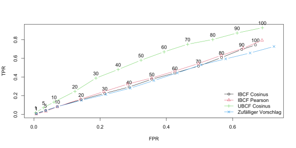
7. Batsman’s Sixes

The snippet of code estimes the sixes of the batsman against bowlers. The ROC and AUC curve for UBCF looks a lot better here, as it significantly greater than 0.5

df3 <- select(df, batsman1,bowler1,sixes)
df6 <- xtabs(sixes ~ ., df3)
df7 <- as.data.frame.matrix(df6)
df8 <- data.matrix(df7)
df8[df8 == 0] <- NA
r <- as(df8,"realRatingMatrix")
r0=r[(rowCounts(r) > 10),]
getRatingMatrix(r0)[1:10,1:10]


## 10 x 10 sparse Matrix of class "dgCMatrix"


##    [[ suppressing 10 column names 'A Mishra', 'A Nortje', 'A Zampa' ... ]]


##                                      
## AB de Villiers  3 3 . . . 18 .  3 . .
## AD Russell      3 . . . .  . . 12 . .
## AJ Finch        2 . . . .  . .  . . .
## AM Rahane       7 . . . .  3 1  . . .
## AR Patel        4 . 3 . .  6 .  1 . .
## AT Rayudu       5 2 . . .  . .  1 . .
## BA Stokes       . . . . .  . .  . . .
## CA Lynn         . . . . .  . .  9 . .
## CH Gayle       17 . . . . 17 .  . . .
## CH Morris       . . 3 . .  . .  . . .


summary(getRatings(r0))


##    Min. 1st Qu.  Median    Mean 3rd Qu.    Max. 
##    1.00    3.00    3.00    4.68    6.00   33.00


evalRecomMethods(r0[1:dim(r0)[1]],k1=5,given=7,goodRating1=median(getRatings(r0)))


## Timing stopped at: 0.003 0 0.002

a=eval(r0[1:dim(r0)[1]],0.8, k1=5,given1=7,goodRating1=median(getRatings(r0)),"UBCF")


## Recommender of type 'UBCF' for 'realRatingMatrix' 
## learned using 52 users.
## 14 x 145 rating matrix of class 'realRatingMatrix' with 1634 ratings.
##      RMSE       MSE       MAE 
##  3.529922 12.460350  2.532122


b=round(as(a,"matrix")[1:10,1:10])
c <- as(b,"realRatingMatrix")
o=as(c,"data.frame")
names(o) =c("batsman","bowler","Sixes")

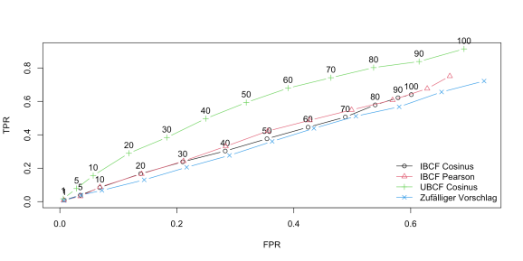
8. Batsman’s Fours

The code below estimates 4s for the batsmen

df3 <- select(df, batsman1,bowler1,fours)
df6 <- xtabs(fours ~ ., df3)
df7 <- as.data.frame.matrix(df6)
df8 <- data.matrix(df7)
df8[df8 == 0] <- NA
r <- as(df8,"realRatingMatrix")
r0=r[(rowCounts(r) > 10),]
getRatingMatrix(r0)[1:10,1:10]


## 10 x 10 sparse Matrix of class "dgCMatrix"


##    [[ suppressing 10 column names 'A Mishra', 'A Nortje', 'A Zampa' ... ]]


##                                      
## AB de Villiers   . 1 . . . 24 . 3 . .
## Abhishek Sharma  . . . . .  . . . . .
## AD Russell       1 . . . .  . . 9 . .
## AJ Finch         . 1 . . .  3 2 . . .
## AK Markram       . . . . .  . . . . .
## AM Rahane       11 . . . .  8 7 . . 3
## AR Patel         . . . . .  . . 3 . .
## AT Rayudu       11 2 3 . .  6 . 6 . .
## BA Stokes        1 . . . .  . . . . .
## CA Lynn          . . . . .  . . 6 . .


summary(getRatings(r0))


##    Min. 1st Qu.  Median    Mean 3rd Qu.    Max. 
##   1.000   3.000   4.000   6.339   9.000  55.000


evalRecomMethods(r0[1:dim(r0)[1]],k1=5,given=7,goodRating1=median(getRatings(r0)))


## Timing stopped at: 0.008 0 0.008


## Warning in .local(x, method, ...): 
##   Recommender 'UBCF Pearson' has failed and has been removed from the results!

a=eval(r0[1:dim(r0)[1]],0.8, k1=5,given1=7,goodRating1=median(getRatings(r0)),"UBCF")


## Recommender of type 'UBCF' for 'realRatingMatrix' 
## learned using 67 users.
## 17 x 145 rating matrix of class 'realRatingMatrix' with 2083 ratings.
##      RMSE       MSE       MAE 
##  5.486661 30.103447  4.060990


b=round(as(a,"matrix")[1:10,1:10])
c <- as(b,"realRatingMatrix")
p=as(c,"data.frame")
names(p) =c("batsman","bowler","Fours")

9. Batsman’s Total Runs

The code below estimates the total runs that would have scored by the batsman against different bowlers

df3 <- select(df, batsman1,bowler1,totalRuns)
df6 <- xtabs(totalRuns ~ ., df3)
df7 <- as.data.frame.matrix(df6)
df8 <- data.matrix(df7)
df8[df8 == 0] <- NA
r <- as(df8,"realRatingMatrix")
r0=r[(rowCounts(r) > 10),]
getRatingMatrix(r)[1:10,1:10]


## 10 x 10 sparse Matrix of class "dgCMatrix"


##    [[ suppressing 10 column names 'A Mishra', 'A Nortje', 'A Zampa' ... ]]


##                                          
## A Badoni         .  . . . .   . .   . . .
## A Manohar        .  . . . .   . .   . . .
## A Nortje         .  . . . .   . .   . . .
## AB de Villiers  61 36 3 . 6 261 .  69 . .
## Abdul Samad      . 57 . . .  12 .   . . .
## Abhishek Sharma  3  . . . .   6 .   . . .
## AD Russell      39  . . . .   . . 129 . .
## AF Milne         .  . . . .   . .   . . .
## AJ Finch        15  7 . . 3  18 9   . . .
## AJ Tye           .  . . . .   . 4   . . .


summary(getRatings(r0))


##    Min. 1st Qu.  Median    Mean 3rd Qu.    Max. 
##    1.00    9.00   24.00   41.36   54.00  452.00


evalRecomMethods(r0[1:dim(r0)[1]],k1=5,given1=7,goodRating1=median(getRatings(r0)))

a=eval(r0[1:dim(r0)[1]],0.8, k1=5,given1=7,goodRating1=median(getRatings(r0)),"UBCF")


## Recommender of type 'UBCF' for 'realRatingMatrix' 
## learned using 105 users.
## 27 x 145 rating matrix of class 'realRatingMatrix' with 3256 ratings.
##       RMSE        MSE        MAE 
##   41.50985 1723.06788   29.52958


b=round(as(a,"matrix")[1:10,1:10])
c <- as(b,"realRatingMatrix")
q=as(c,"data.frame")
names(q) =c("batsman","bowler","TotalRuns")

10. Batsman’s Balls Faced

The snippet estimates the balls faced by batsmen versus bowlers

df3 <- select(df, batsman1,bowler1,ballsFaced)
df6 <- xtabs(ballsFaced ~ ., df3)
df7 <- as.data.frame.matrix(df6)
df8 <- data.matrix(df7)
df8[df8 == 0] <- NA
r <- as(df8,"realRatingMatrix")
r0=r[(rowCounts(r) > 10),]
getRatingMatrix(r)[1:10,1:10]


## 10 x 10 sparse Matrix of class "dgCMatrix"


##    [[ suppressing 10 column names 'A Mishra', 'A Nortje', 'A Zampa' ... ]]


##                                         
## A Badoni         .  . . . .   . .  . . .
## A Manohar        .  . . . .   . .  . . .
## A Nortje         .  . . . .   . .  . . .
## AB de Villiers  63 21 9 . 9 117 . 63 . .
## Abdul Samad      . 25 . . .  12 .  . . .
## Abhishek Sharma  2  . . . .   9 .  . . .
## AD Russell      35  . . . .   . . 66 . .
## AF Milne         .  . . . .   . .  . . .
## AJ Finch         6  6 . . 6  21 8  . . .
## AJ Tye           .  . . . .   9 4  . . .


summary(getRatings(r0))


##    Min. 1st Qu.  Median    Mean 3rd Qu.    Max. 
##    1.00    9.00   18.00   30.21   39.00  384.00


evalRecomMethods(r0[1:dim(r0)[1]],k1=5,given=7,goodRating1=median(getRatings(r0)))

a=eval(r0[1:dim(r0)[1]],0.8, k1=5,given1=7,goodRating1=median(getRatings(r0)),"UBCF")


## Recommender of type 'UBCF' for 'realRatingMatrix' 
## learned using 112 users.
## 28 x 145 rating matrix of class 'realRatingMatrix' with 3378 ratings.
##       RMSE        MSE        MAE 
##   33.91251 1150.05835   23.39439


b=round(as(a,"matrix")[1:10,1:10])
c <- as(b,"realRatingMatrix")
r=as(c,"data.frame")
names(r) =c("batsman","bowler","BallsFaced")

11. Generate the Batsmen Performance Estimate

This code generates the estimated dataframe with known and ‘predicted’ values

a1=merge(m,n,by=c("batsman","bowler"))
a2=merge(a1,o,by=c("batsman","bowler"))
a3=merge(a2,p,by=c("batsman","bowler"))
a4=merge(a3,q,by=c("batsman","bowler"))
a5=merge(a4,r,by=c("batsman","bowler"))
a6= select(a5, batsman,bowler,BallsFaced,TotalRuns,Fours, Sixes, SR,TimesOut)
head(a6)


##          batsman          bowler BallsFaced TotalRuns Fours Sixes  SR TimesOut
## 1 AB de Villiers        A Mishra         94       124     7     5 144        5
## 2 AB de Villiers        A Nortje         26        42     4     3 148        3
## 3 AB de Villiers         A Zampa         28        42     5     7 106        4
## 4 AB de Villiers Abhishek Sharma         22        28     0    10 136        5
## 5 AB de Villiers      AD Russell         70       135    14    12 207        4
## 6 AB de Villiers        AF Milne         31        45     6     6 130        3

12. Bowler analysis

Just like the batsman performance estimation we can consider the bowler’s performances also for estimation. Consider the following table

As in the batsman analysis, for every batsman a set of features like (“strong backfoot player”, “360 degree player”,“Power hitter”) can be estimated with a set of initial values. Also every bowler will have an associated parameter vector θθ. Different bowlers will have performance data for different set of batsmen. Based on the initial estimate of the features and the parameters, gradient descent can be used to minimize actual values {for e.g. wicketsTaken(ratings)}.

load("recom_data/bowlerVsBatsman20_22.rdata")

12a. Bowler dataframe

Inspecting the bowler dataframe

head(df2)


##    bowler1        batsman1 balls runsConceded       ER wicketTaken
## 1 A Mishra        A Badoni     0            0 0.000000           0
## 2 A Mishra       A Manohar     0            0 0.000000           0
## 3 A Mishra        A Nortje     0            0 0.000000           0
## 4 A Mishra  AB de Villiers    63           61 5.809524           0
## 5 A Mishra     Abdul Samad     0            0 0.000000           0
## 6 A Mishra Abhishek Sharma     2            3 9.000000           0


names(df2)


## [1] "bowler1"      "batsman1"     "balls"        "runsConceded" "ER"          
## [6] "wicketTaken"

13. Balls bowled by bowler

The below section estimates the balls bowled for each bowler. We can see that UBCF Pearson and UBCF Cosine both perform well

df3 <- select(df2, bowler1,batsman1,balls)
df6 <- xtabs(balls ~ ., df3)
df7 <- as.data.frame.matrix(df6)
df8 <- data.matrix(df7)
df8[df8 == 0] <- NA
r <- as(df8,"realRatingMatrix")
r0=r[(rowCounts(r) > 10),]
getRatingMatrix(r0)[1:10,1:10]


## 10 x 10 sparse Matrix of class "dgCMatrix"


##    [[ suppressing 10 column names 'A Badoni', 'A Manohar', 'A Nortje' ... ]]


##                                          
## A Mishra        . . .  63  .  2 35 .  6 .
## A Nortje        . . .  21 25  .  . .  6 .
## A Zampa         . . .   9  .  .  . .  . .
## Abhishek Sharma . . .   9  .  .  . .  6 .
## AD Russell      . . . 117 12  9  . . 21 9
## AF Milne        . . .   .  .  .  . .  8 4
## AJ Tye          . . .  63  .  . 66 .  . .
## Akash Deep      . . .   .  .  .  . .  . .
## AR Patel        . . . 188  5  1 84 . 29 5
## Arshdeep Singh  . . .   6  6 24 18 . 12 .


summary(getRatings(r0))


##    Min. 1st Qu.  Median    Mean 3rd Qu.    Max. 
##    1.00    9.00   18.00   29.61   36.00  384.00


evalRecomMethods(r0[1:dim(r0)[1]],k1=5,given=7,goodRating1=median(getRatings(r0)))

a=eval(r0[1:dim(r0)[1]],0.8,k1=5,given1=7,goodRating1=median(getRatings(r0)),"UBCF")


## Recommender of type 'UBCF' for 'realRatingMatrix' 
## learned using 96 users.
## 24 x 195 rating matrix of class 'realRatingMatrix' with 3954 ratings.
##      RMSE       MSE       MAE 
##  30.72284 943.89294  19.89204


b=round(as(a,"matrix")[1:10,1:10])
c <- as(b,"realRatingMatrix")
s=as(c,"data.frame")
names(s) =c("bowler","batsman","BallsBowled")

14. Runs conceded by bowler

This section estimates the runs conceded by the bowler. The UBCF Cosinus algorithm performs the best with TPR increasing fastewr than FPR

df3 <- select(df2, bowler1,batsman1,runsConceded)
df6 <- xtabs(runsConceded ~ ., df3)
df7 <- as.data.frame.matrix(df6)
df8 <- data.matrix(df7)
df8[df8 == 0] <- NA
r <- as(df8,"realRatingMatrix")
r0=r[(rowCounts(r) > 10),]
getRatingMatrix(r0)[1:10,1:10]


## 10 x 10 sparse Matrix of class "dgCMatrix"


##    [[ suppressing 10 column names 'A Badoni', 'A Manohar', 'A Nortje' ... ]]


##                                            
## A Mishra        . . .  61  .  3  41 . 15  .
## A Nortje        . . .  36 57  .   . .  8  .
## A Zampa         . . .   3  .  .   . .  .  .
## Abhishek Sharma . . .   6  .  .   . .  3  .
## AD Russell      . . . 276 12  6   . . 21  .
## AF Milne        . . .   .  .  .   . . 10  4
## AJ Tye          . . .  69  .  . 138 .  .  .
## Akash Deep      . . .   .  .  .   . .  .  .
## AR Patel        . . . 205  5  . 165 . 33 13
## Arshdeep Singh  . . .  18  3 51  51 .  6  .


summary(getRatings(r0))


##    Min. 1st Qu.  Median    Mean 3rd Qu.    Max. 
##    1.00    9.00   24.00   41.34   54.00  458.00


evalRecomMethods(r0[1:dim(r0)[1]],k1=5,given=7,goodRating1=median(getRatings(r0)))


## Timing stopped at: 0.004 0 0.004


## Warning in .local(x, method, ...): 
##   Recommender 'UBCF Pearson' has failed and has been removed from the results!

a=eval(r0[1:dim(r0)[1]],0.8,k1=5,given1=7,goodRating1=median(getRatings(r0)),"UBCF")


## Recommender of type 'UBCF' for 'realRatingMatrix' 
## learned using 95 users.
## 24 x 195 rating matrix of class 'realRatingMatrix' with 3820 ratings.
##       RMSE        MSE        MAE 
##   43.16674 1863.36749   30.32709


b=round(as(a,"matrix")[1:10,1:10])
c <- as(b,"realRatingMatrix")
t=as(c,"data.frame")
names(t) =c("bowler","batsman","RunsConceded")

15. Economy Rate of the bowler

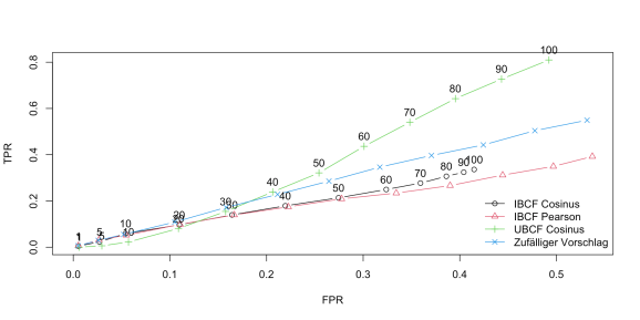
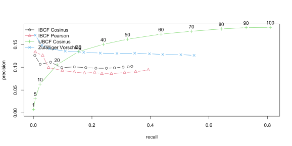
This section computes the economy rate of the bowler. The performance is not all that good

df3 <- select(df2, bowler1,batsman1,ER)
df6 <- xtabs(ER ~ ., df3)
df7 <- as.data.frame.matrix(df6)
df8 <- data.matrix(df7)
df8[df8 == 0] <- NA
r <- as(df8,"realRatingMatrix")
r0=r[(rowCounts(r) > 10),]
getRatingMatrix(r0)[1:10,1:10]


## 10 x 10 sparse Matrix of class "dgCMatrix"


##    [[ suppressing 10 column names 'A Badoni', 'A Manohar', 'A Nortje' ... ]]


##                                                                       
## A Mishra        . . .  5.809524  .     9.00  7.028571 . 15.000000  .  
## A Nortje        . . . 10.285714 13.68  .     .        .  8.000000  .  
## A Zampa         . . .  2.000000  .     .     .        .  .         .  
## Abhishek Sharma . . .  4.000000  .     .     .        .  3.000000  .  
## AD Russell      . . . 14.153846  6.00  4.00  .        .  6.000000  .  
## AF Milne        . . .  .         .     .     .        .  7.500000  6.0
## AJ Tye          . . .  6.571429  .     .    12.545455 .  .         .  
## Akash Deep      . . .  .         .     .     .        .  .         .  
## AR Patel        . . .  6.542553  6.00  .    11.785714 .  6.827586 15.6
## Arshdeep Singh  . . . 18.000000  3.00 12.75 17.000000 .  3.000000  .


summary(getRatings(r0))


##    Min. 1st Qu.  Median    Mean 3rd Qu.    Max. 
##  0.3529  5.2500  7.1126  7.8139  9.8000 36.0000


evalRecomMethods(r0[1:dim(r0)[1]],k1=5,given=7,goodRating1=median(getRatings(r0)))


## Timing stopped at: 0.003 0 0.004


## Warning in .local(x, method, ...): 
##   Recommender 'UBCF Pearson' has failed and has been removed from the results!

a=eval(r0[1:dim(r0)[1]],0.8,k1=5,given1=7,goodRating1=median(getRatings(r0)),"UBCF")


## Recommender of type 'UBCF' for 'realRatingMatrix' 
## learned using 95 users.
## 24 x 195 rating matrix of class 'realRatingMatrix' with 3839 ratings.
##      RMSE       MSE       MAE 
##  4.380680 19.190356  3.316556


b=round(as(a,"matrix")[1:10,1:10])
c <- as(b,"realRatingMatrix")
u=as(c,"data.frame")
names(u) =c("bowler","batsman","EconomyRate")

16. Wickets Taken by bowler

The code below computes the wickets taken by the bowler versus different batsmen

df3 <- select(df2, bowler1,batsman1,wicketTaken)
df6 <- xtabs(wicketTaken ~ ., df3)
df7 <- as.data.frame.matrix(df6)
df8 <- data.matrix(df7)
df8[df8 == 0] <- NA
r <- as(df8,"realRatingMatrix")
r0=r[(rowCounts(r) > 10),]
getRatingMatrix(r0)[1:10,1:10]


## 10 x 10 sparse Matrix of class "dgCMatrix"


##    [[ suppressing 10 column names 'A Badoni', 'A Manohar', 'A Nortje' ... ]]


##                                   
## A Mishra       . . . . . . 1 . . .
## A Nortje       . . . 4 . . . . . .
## A Zampa        . . . 3 . . . . . .
## AD Russell     . . . 3 . . . . . .
## AJ Tye         . . . 3 . . 6 . . .
## AR Patel       . . . 4 . 1 3 . 1 1
## Arshdeep Singh . . . 3 . . 3 . . .
## AS Rajpoot     . . . . . . 3 . . .
## Avesh Khan     . . . . . . 1 . 3 .
## B Kumar        . . . 9 . . 3 . 1 .


summary(getRatings(r0))


##    Min. 1st Qu.  Median    Mean 3rd Qu.    Max. 
##   1.000   3.000   3.000   3.423   3.000  21.000


evalRecomMethods(r0[1:dim(r0)[1]],k1=5,given=7,goodRating1=median(getRatings(r0)))


## Timing stopped at: 0.003 0 0.003


## Warning in .local(x, method, ...): 
##   Recommender 'UBCF Pearson' has failed and has been removed from the results!

a=eval(r0[1:dim(r0)[1]],0.8,k1=5,given1=7,goodRating1=median(getRatings(r0)),"UBCF")


## Recommender of type 'UBCF' for 'realRatingMatrix' 
## learned using 64 users.
## 16 x 195 rating matrix of class 'realRatingMatrix' with 1908 ratings.
##     RMSE      MSE      MAE 
## 2.672677 7.143203 1.956934


b=round(as(a,"matrix")[1:10,1:10])
c <- as(b,"realRatingMatrix")
v=as(c,"data.frame")
names(v) =c("bowler","batsman","WicketTaken")

17. Generate the Bowler Performance estmiate

The entire dataframe is regenerated with known and ‘predicted’ values

r1=merge(s,t,by=c("bowler","batsman"))
r2=merge(r1,u,by=c("bowler","batsman"))
r3=merge(r2,v,by=c("bowler","batsman"))
r4= select(r3,bowler, batsman, BallsBowled,RunsConceded,EconomyRate, WicketTaken)
head(r4)


##     bowler         batsman BallsBowled RunsConceded EconomyRate WicketTaken
## 1 A Mishra  AB de Villiers         102          144           8           4
## 2 A Mishra     Abdul Samad          13           20           7           4
## 3 A Mishra Abhishek Sharma          14           26           8           2
## 4 A Mishra      AD Russell          47           85           9           3
## 5 A Mishra        AJ Finch          45           61          11           4
## 6 A Mishra          AJ Tye          14           20           5           4

18. Conclusion

This post showed an approach for performing the Batsmen Performance Estimate & Bowler Performance Estimate. The performance of the recommender engine could have been better. In any case, I think this approach will work for player estimation provided the recommender algorithm is able to achieve a high degree of accuracy. This will be a good way to estimate as the algorithm will be able to determine features and nuances of batsmen and bowlers which cannot be captured by data.

References

Also see

To see all posts click Index of posts

To leave a comment for the author, please follow the link and comment on their blog: R – Giga thoughts ….

R-bloggers.com offers daily e-mail updates about R news and tutorials about learning R and many other topics. Click here if you're looking to post or find an R/data-science job.

Want to share your content on R-bloggers? click here if you have a blog, or here if you don't.

R-bloggers

R news and tutorials contributed by hundreds of R bloggers

Player Performance Estimation using AI Collaborative Filtering

1. Introduction

Problem statement

1a. A note on ROC and Precision-Recall curves

2. Define recommender lab helper functions

3. Batsman performance estimation

3a. Batting dataframe

3b Data set and data preparation

3c. Exploratory analysis

4. Create a visual representation of the rating data before and after the normalization

4a. Data for analysis

5. Batsman’s times Out

6. Batsman’s Strike rate

7. Batsman’s Sixes

8. Batsman’s Fours

9. Batsman’s Total Runs

10. Batsman’s Balls Faced

11. Generate the Batsmen Performance Estimate

12. Bowler analysis

12a. Bowler dataframe

13. Balls bowled by bowler

14. Runs conceded by bowler

15. Economy Rate of the bowler

16. Wickets Taken by bowler

17. Generate the Bowler Performance estmiate

18. Conclusion

References

Also see

Related

1. Introduction

Problem statement

1a. A note on ROC and Precision-Recall curves

2. Define recommender lab helper functions

3. Batsman performance estimation

3a. Batting dataframe

3b Data set and data preparation

3c. Exploratory analysis

4. Create a visual representation of the rating data before and after the normalization

4a. Data for analysis

5. Batsman’s times Out

6. Batsman’s Strike rate

7. Batsman’s Sixes

8. Batsman’s Fours

9. Batsman’s Total Runs

10. Batsman’s Balls Faced

11. Generate the Batsmen Performance Estimate

12. Bowler analysis

12a. Bowler dataframe

13. Balls bowled by bowler

14. Runs conceded by bowler

15. Economy Rate of the bowler

16. Wickets Taken by bowler

17. Generate the Bowler Performance estmiate

18. Conclusion

References

Also see

Related

Never miss an update! Subscribe to R-bloggers to receive e-mails with the latest R posts. (You will not see this message again.)

Never miss an update!
Subscribe to R-bloggers to receive
e-mails with the latest R posts.
(You will not see this message again.)