
Deriving the Supply Curve from the Profit Function in R
Want to share your content on R-bloggers? click here if you have a blog, or here if you don't.

In this blog post we will discuss the derivation of a microfounded supply curve in R.
Specifically we are interested in seeing how we can compute the supply curve from our firms objective problem. In this case we will consider solving for the supply curve from the following profit function:
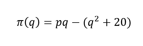
We note that in this particular example we don’t define our production technology directly, but rather use a cost function which is defined in terms of quantity. This will be key in computing our supply curve. The code which is used to generate this supply curve is given below:
################################
#Deriving the Supply Curve in R#
################################
#Starting Values
prices<-seq(1,15,by=0.1)
q0<-c(1)
qsupply<-NULL
#Profit function
profitfunc<-function(q){
return(p*q-q^2-20)
}
#For Loop
for(p in prices){
cmin<-optim(q0,
profitfunc,
control= list(fnscale=-1),
lower=0,
method = "L-BFGS-B")
q<-cmin$par[1]
qsupply<-rbind(qsupply,q)}
#Plot supply curve
df<-data.frame(qsupply,prices)
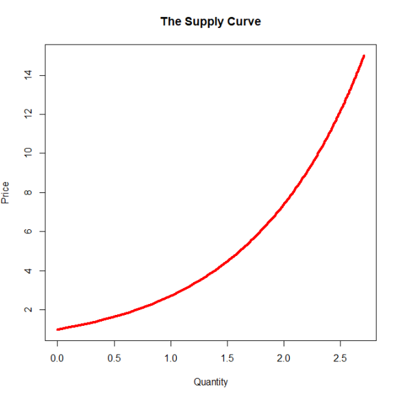
plot(df$qsupply,df$prices,xlab="Quantity",ylab="Price", main="The Supply Curve",
col='red', lwd=4.0, type="l")
Some things which are worth noting from this code:
- The function which does most of the work for us is
optim(). The defaults of this function is to search for a minimum so we need to tell the function we are looking for a maximum. The way we do this is through the use of the argumentcontrol= list(fnscale=-1). - We specify purposely that we are seeking quantities that are positive numbers (there may be circumstances where our profit function is maximized under negative inputs). To rule out these cases we define our lower limit of
qto be0with the argumentlower=0. - We can define much more complex sort of supply functions depending on how our costs enter our profit function. Consider the case of where our profit function is now:
profitfunc<-function(q){
  return(-p*q+exp(q)+20)
}
From this function we get a convex supply curve
There could be more shapes which we can generate, but i’ll leave that to the more creative coder. In the next blogs we will finally discuss how we can compute a simple general equilibrium model.
R-bloggers.com offers daily e-mail updates about R news and tutorials about learning R and many other topics. Click here if you're looking to post or find an R/data-science job.
Want to share your content on R-bloggers? click here if you have a blog, or here if you don't.