
RObservations #29 – Classifying and Filtering Coordinates By Using the sf Library
Want to share your content on R-bloggers? click here if you have a blog, or here if you don't.

Introduction
Geo-spatial analysis and visualizations is a powerful tool for providing insight bringing an idea or a result in a more tangible manner. Oftentimes, we are only interested in a specific points or we wan to classify the data we have by a larger location it belongs to. In this blog I share my discovery of the sf library’s st_intersects() function and how its possible to use it to classify and filter longitude and latitude data points within given multipolygons.
The Data
The data which I’m going to use comes from latlong.net where I took some random longitudes and latitudes of locations in Canada and copied them into a data frame. The data looks like this:
head(locations)


##   Latitude Longitude
## 1 51.21389 -102.4628
## 2 52.32194 -106.5842
## 3 50.28805 -107.7939
## 4 52.75750 -108.2861
## 5 50.39333 -105.5519
## 6 50.93056 -102.8078
Now to plot the data on a map we are going to need to create a map of Canada. The rnaturalearth package is a really useful package for this as it provides necessary polygon data for plotting provinces and states world wide. The code for plotting a map of Canada with the relevant points is:
library(tidyverse)
library(sf)
library(rnaturalearth)
# Canadian Provinces
provinceData<- ne_states("canada") %>% st_as_sf()
# Map of Canada
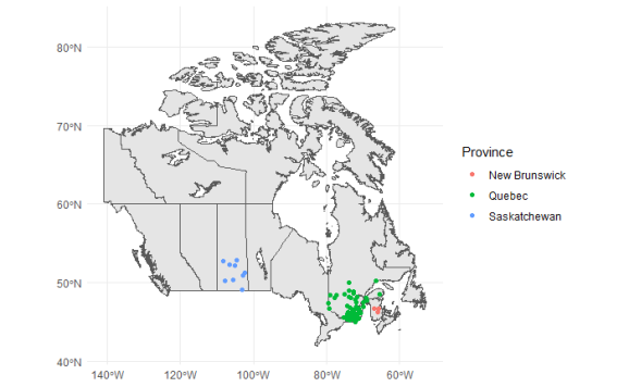
ggplot()+
geom_sf(data=provinceData)+
geom_sf(data=locations %>% st_as_sf(coords = c("Longitude", "Latitude"), crs = 4326))+
theme_minimal()

It appears that there is a erroneously entered point plotted here as well as data on points in Saskatchewan, Quebec and New Brunswick. We can use the sf_intersects method to classify and filter the data accordingly.
Classifying/Filtering the Data
For classifying the data, first lets isolate the specific polygons of the provinces of interest. It is with this that we can apply the st_intersects() function to determine which points belong in which province and have an index to label the points accordingly.
The code I use for doing this is:
# Using Magrittr for the exploding pipe operator
library(magrittr)

# Isolating specific polygons
saskatchewanPolygons<- provinceData %>% filter(name_id=="Saskatchewan") %$% geometry
quebecPolygons <- provinceData %>% filter(name_id=="Quebec") %$% geometry
newBrunswickPolygons<-provinceData %>% filter(name_id=="New Brunswick") %$% geometry


# Getting the indices
saskatchewanIndex<-locations %>%
                   st_as_sf(coords = c("Longitude", "Latitude"), crs = 4326) %$% geometry %>%
                   st_intersects(saskatchewanPolygons) %>%
                   lapply(function(x) ifelse(length(x)==0,FALSE,TRUE)) %>%
                   unlist()

quebecIndex <- locations %>%
                   st_as_sf(coords = c("Longitude", "Latitude"), crs = 4326) %$% geometry %>%
                   st_intersects(quebecPolygons) %>%
                   lapply(function(x) ifelse(length(x)==0,FALSE,TRUE)) %>%
                   unlist()

newBrunswickIndex<-locations %>%
                   st_as_sf(coords = c("Longitude", "Latitude"), crs = 4326) %$% geometry %>%
                   st_intersects(newBrunswickPolygons) %>%
                   lapply(function(x) ifelse(length(x)==0,FALSE,TRUE)) %>%
                   unlist()


# Using a Base R approach
# Create a new column
locations$Province <- c()
locations$Province[saskatchewanIndex]<-"Saskatchewan"
locations$Province[quebecIndex]<-"Quebec"
locations$Province[newBrunswickIndex]<-"New Brunswick"
Now that the data has been transformed accordingly its possible to plot the points and color them by Province. For aesthetic reasons, I remove the NA values as well.
ggplot()+
geom_sf(data=provinceData)+
geom_sf(data=locations %>%
          # Filtering NA values out
          filter(!is.na(Province)) %>%
          st_as_sf(coords = c("Longitude", "Latitude"), crs = 4326),
        mapping=aes(color=Province))+
theme_minimal()
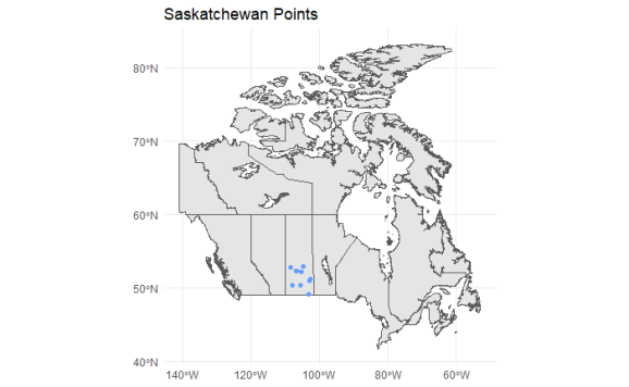
It goes without saying, now that the data has been labeled by Province, it can also be filtered with a simple filter() command.
ggplot()+
geom_sf(data=provinceData)+
geom_sf(data=locations %>%
          filter(Province=="Saskatchewan") %>%
          st_as_sf(coords = c("Longitude", "Latitude"), crs = 4326),
        color="#619CFF")+
  ggtitle("Saskatchewan Points")+
  theme_minimal()
Conclusion
The sf library is a library that I haven’t really explored until recently and the functions available provide really powerful tools for analyzing and wragling spatial data. If you have the time, be sure to check out the rnaturalearth package as well for getting the multipolygon data that you need for producing maps with ease.
Thank you for checking out this blog! Be sure to subscribe to never miss an update!

Want to see more of my content?
Be sure to subscribe and never miss an update!
R-bloggers.com offers daily e-mail updates about R news and tutorials about learning R and many other topics. Click here if you're looking to post or find an R/data-science job.
Want to share your content on R-bloggers? click here if you have a blog, or here if you don't.